17–34. (20 min.) Sales Activity Variance—Service Organization: K&B.
Flexible Budget
(based on
actual of
7,200 hours)
Sales
Activity
Variance
Master Budget
(based on
budgeted 9,000
hours)
Revenue …………………………..
$648,000
$162,000
U
$810,000
80,000
F
F
F
$720,000
17–35. (30 min.) Profit Variance Analysis—Service Organization: K&B.
(1)
(2)
(3)
(4)
(5)
(6)
Actual
(7,200 hrs.)
Cost
Variances
Price
Variances
Flexible
Budget
(7,200 hrs.)
Sales
Activity
Variance
Master
Budget
(9,000 hrs.)
Revenue ………………..
$670,000
$22,000 F
$648,000
$162,000 U
$810,000
Professional salaries .
340,000
$20,000 U
320,000
80,000 F
400,000
Other variable costs ..
24,000 F
Fixed costs …………….
Profit ……………………..
$27,000 U
$22,000 F
$ 90,000
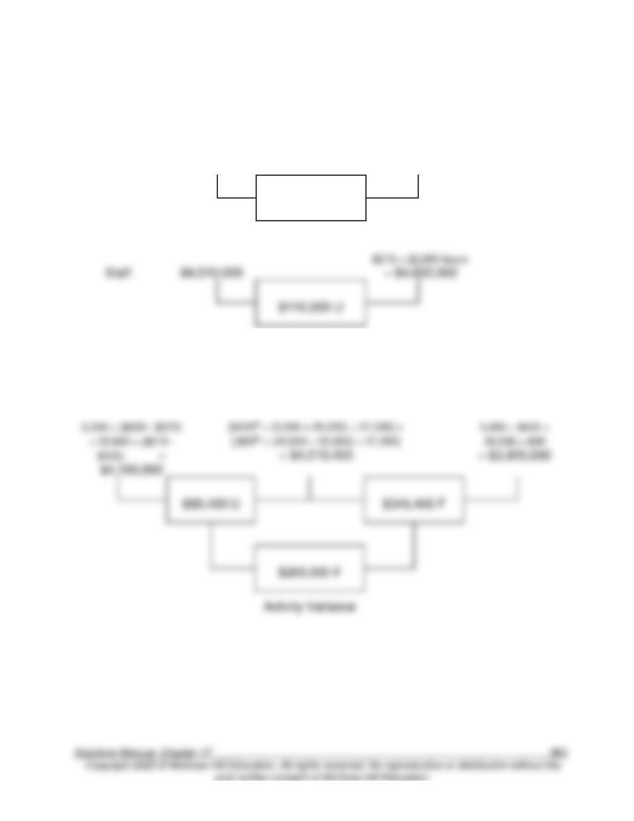
17–36. (20 min.) Sales Price and Activity Variances: EZ-Tax.
Actual
(AP × AQ)
Price Variance
Flexible Budget
(SP × AQ)
Partner
$4,264,000
$800 × 5,200 hours
= $4,160,000
$104,000 F
$4,510,000
Flexible
Budget
Master Budget
AQ × (SP –
SV)
Mix Variance
(SP – SV) × ASQ
Quantity
Variance
SQ × (SP – SV)
$265,000 F
a $425 = $800 – $375.
b $90 = $210 – $120.
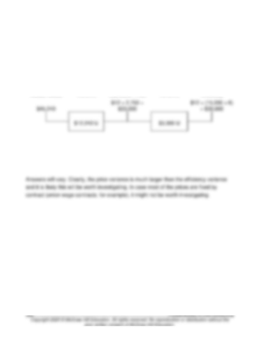
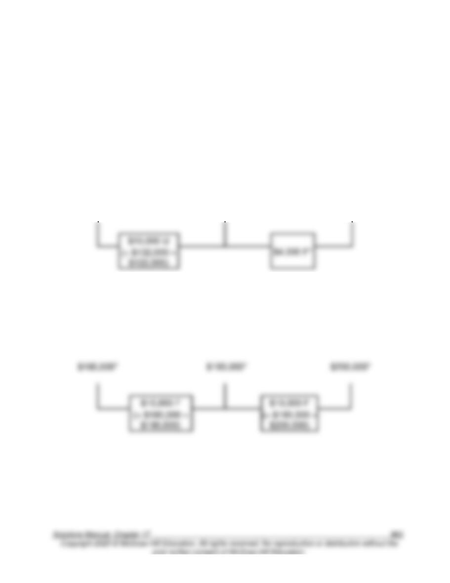
17–37. (10 min.) Investigating Variances: Harry’s Hotel.
Answers will vary. Clearly, the price variances are something to look into. Although they
come close to cancelling out, we would want to understand the causes for the two very
different results. For example, is the “mix” of partners and staff (different levels within each
group) different from what was expected (an input mix variance)? The quantity variance is
worth investigating to see if this suggests greater activity in the future.
17–38. (10 min.) Variable Cost Variances: Harry’s Hotel.
Price
Actual Inputs at
Efficiency
Flexible Budget
(Standard
17–39. (10 min.) Investigating Variances: Harry’s Hotel.
Solutions to Problems
17–40. (20 min.) Prorating Overhead Costs: Parkeville Company.
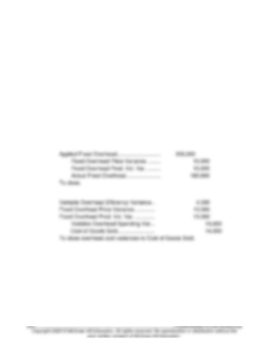
Before recording the variances, we first compute the ones missing from the problem (the
information given is noted with an asterisk; the other numbers are calculated from the
differences):
Variable costs:
Actual
Costs
Spending
Variance
Actual Inputs
at Standard
Price
Efficiency
Variance
Flexible Budget
(Standard
Inputs Allowed
for Good
Output)
$132,000*
$122,000
(= $126,000 – $4,000)
$126,000*
Fixed costs:
Actual
Costs
Price
Variance
Budget
Production
Volume
Variance
Applied
17-40 (continued)
a.
Actual Variable Overhead …………
132,000
Accounts Payable …………….
132,000
To record the purchase of various variable overhead
resources.
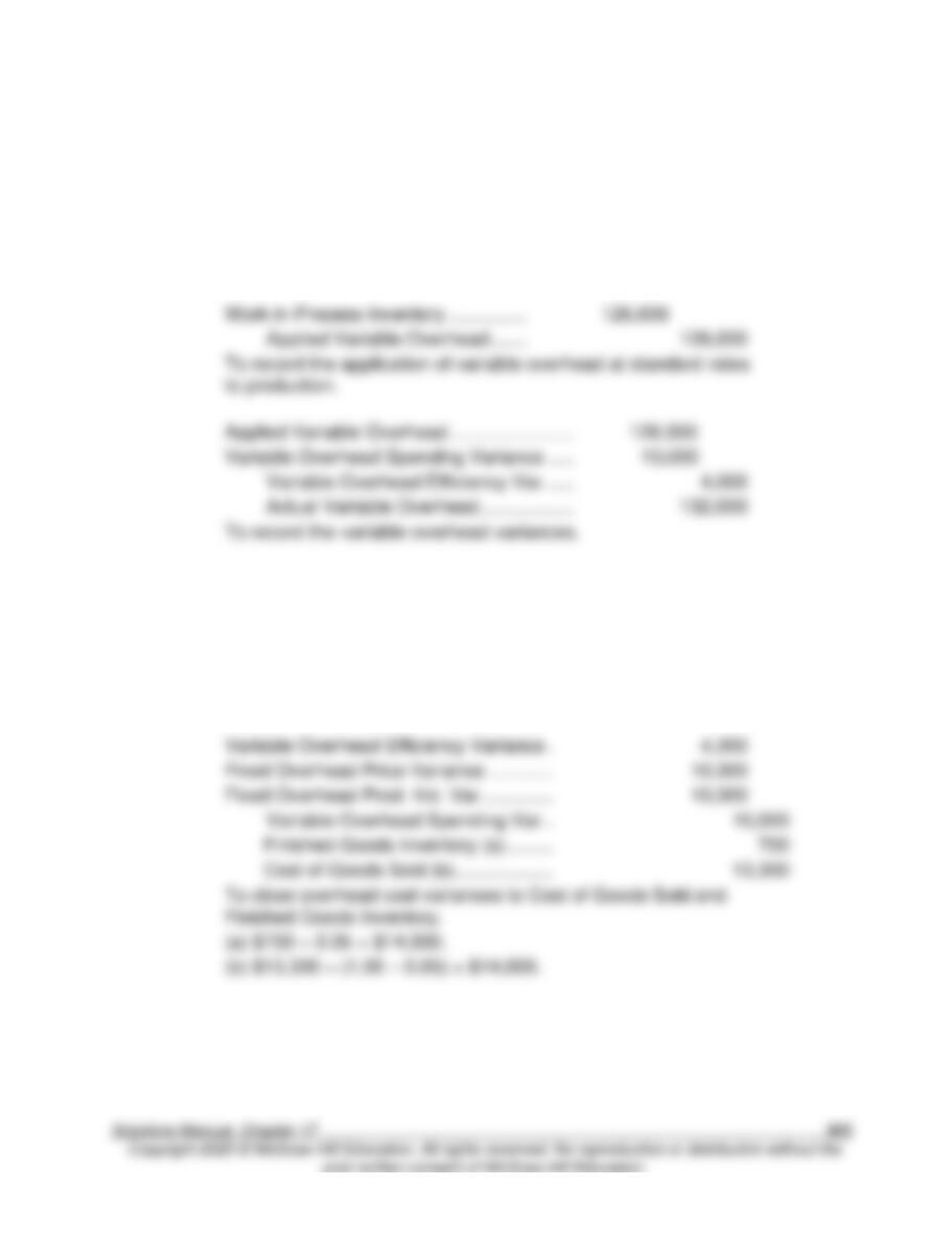
Work-in-Process Inventory ……………
126,000
Applied Variable Overhead ……
126,000
To record the application of variable overhead at standard rates
to production.
Applied Variable Overhead ……………………
126,000
Variable Overhead Spending Variance ……
10,000
Variable Overhead Efficiency Var. …..
4,000
Actual Variable Overhead ………………
132,000
To record the variable overhead variances.
Applied Fixed Overhead ………………………..
Fixed Overhead Price Variance. ……..
Fixed Overhead Prod. Vol. Var. ………
Actual Fixed Overhead …………………..
To close.
Variable Overhead Efficiency Variance ..
Fixed Overhead Price Variance. …………
Fixed Overhead Prod. Vol. Var. ………….
Variable Overhead Spending Var. ..
To close overhead cost variances to Cost of Goods Sold.
17-40 (continued)
b. Finished Goods Inventory is 5 percent of production.
Actual Variable Overhead ………….
132,000
Accounts Payable ……………..
132,000
To record the purchase of various variable overhead
resources.
Applied Variable Overhead …….
Applied Variable Overhead ……………………
Variable Overhead Spending Variance …..
Variable Overhead Efficiency Var. …..
Actual Variable Overhead ………………
To record the variable overhead variances.
Applied Fixed Overhead ……………………….
200,000
Fixed Overhead Price Variance. ……..
10,000
Fixed Overhead Prod. Vol. Var. ………
10,000
Actual Fixed Overhead ………………….
180,000
To close.
Variable Overhead Efficiency Variance .
Fixed Overhead Price Variance. …………
Fixed Overhead Prod. Vol. Var. ………….
Variable Overhead Spending Var. .
(a) $700 = 0.05 × $14,000.
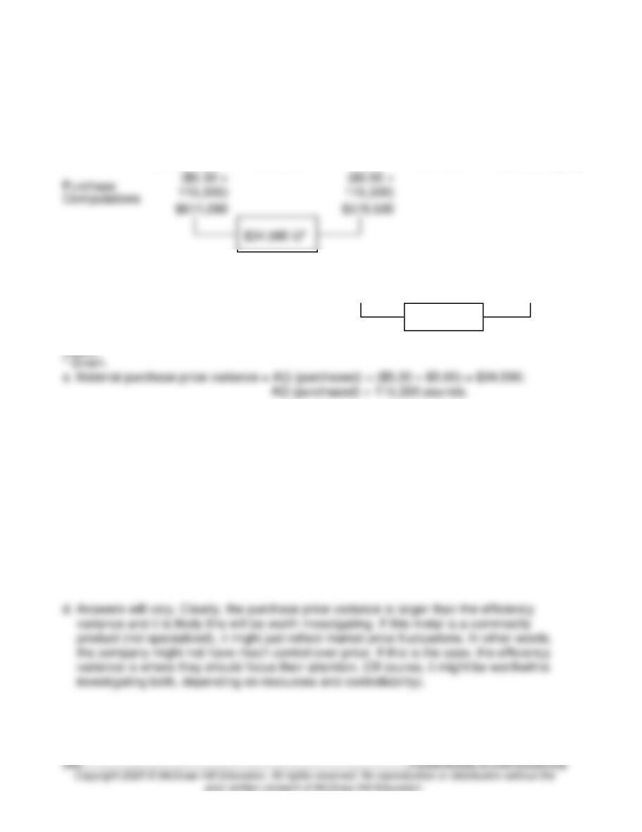
17–41. (20 min.) Variable Cost Variances: Materials Purchased And Used Are Not
Equal: Griffen Company.
Actual Costs
Price
Variance
Actual
Inputs at
Standard
Price
Efficiency
Variance
Flexible Budget
(Standard
Allowed for
Good Output)
$470,000
$5* × 6* ×
15,000*
= $450,000
Usage
Computations
$20,000 U
b. Variable overhead efficiency variance = [AQ (used) – AQ (allowed)] × $2.00 = $8,000 U.
[AQ (used) – (6 × 15,000 units)] × $2.00 = $8,000
U.
AQ (Used) = 94,000 pounds.
Direct material efficiency variance = [AQ (used) – AQ (allowed)] × $5.00
= [94,000 pounds – (6 × 15,000 units)] × $5.00 = $20,000 U.
Alternatively, because the variable overhead application rate is 40 percent (= $2 ÷ $5)
the standard price for materials, and because variable overhead is applied on the basis
of direct materials used, the direct material efficiency variance will be 2.5 (= 1.0 ÷ 0.40)
times the variable overhead efficiency variance.
c. From b, 94,000 pounds were used in August production.
17–42. (20 min.) Industry Volume and Market Share Variances—Missing Data.
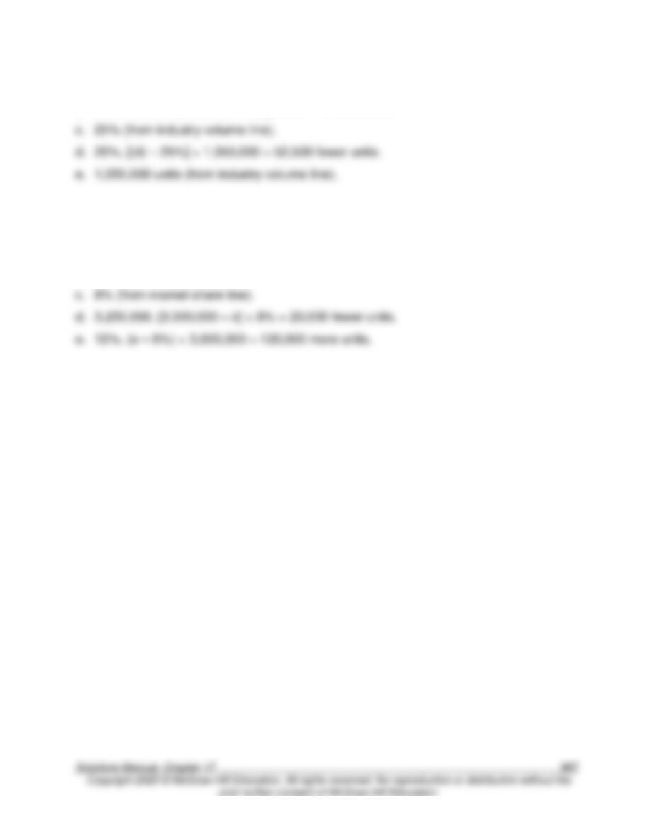
a. 15,000 fewer units = 52,500 fewer units – 37,500 more units.
b. 900,000 units. [1,050,000 – (b)] × 25% = 37,500 units.
17–43. (20 min.) Industry Volume and Market Share—Missing Data.
a. 20,000 fewer units = 100,000 more units activity variance – 120,000 more units market
share variance.
b. 3,000,000 units (from market share line).
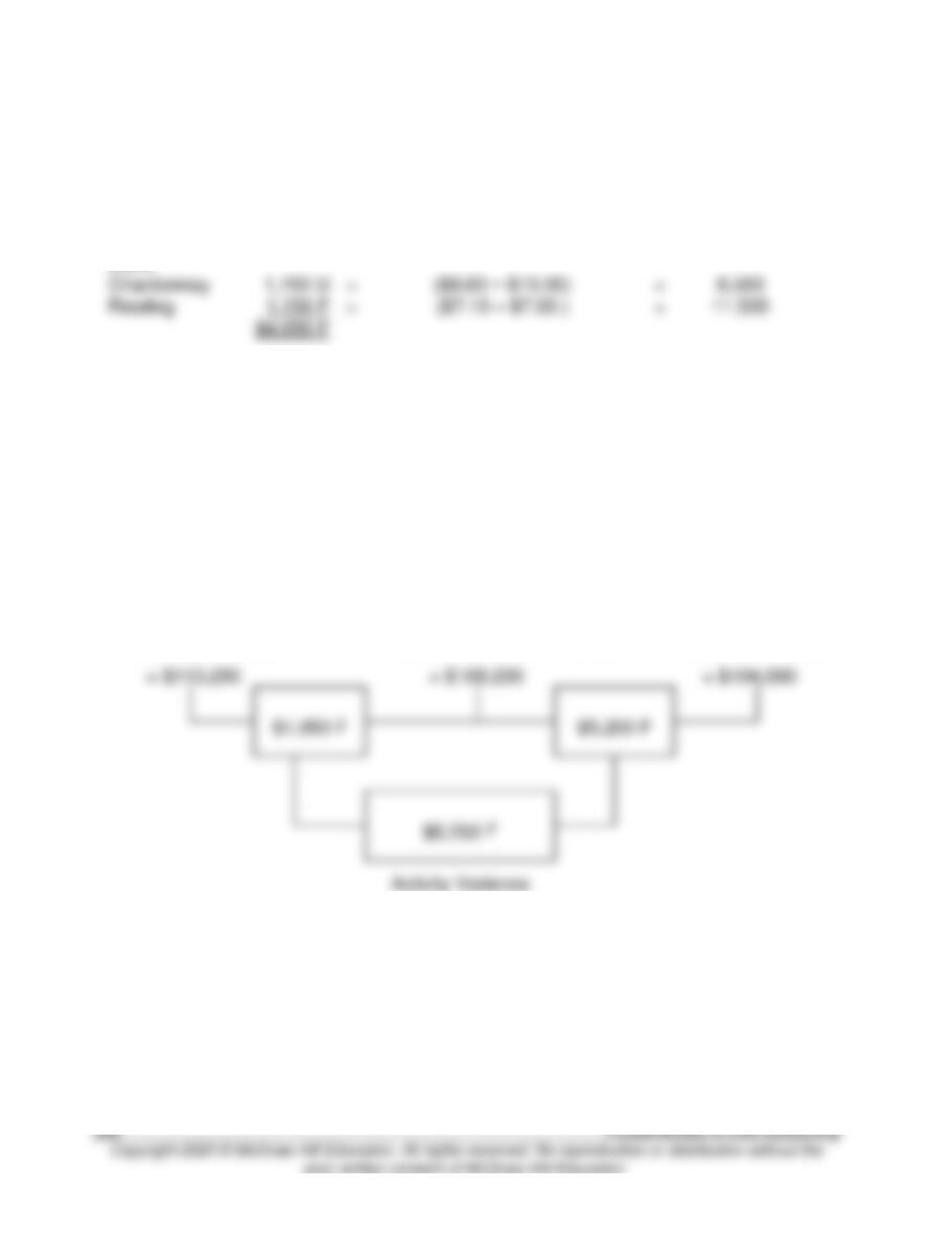
17–44. Sales Mix and Quantity Variances: Lake Cellars.
a. Price Variance = (Actual Price − Budgeted Price) × Actual Quantity:
Variety:
Price
Variance
=
(Actual Price − Budgeted Price)
×
Actual Quantity
Sauvignon
$5,500 F
=
($9.25 − $9.00)
×
22,000
b. and c.
The actual prices are not relevant here. The mix and quantity variances are based on
standard (budgeted) contribution margin per unit.
Flexible Budget
AQ × (SP – SV)
Mix
Variance
ASQ × (SP – SV)
Quantity
Variance
Master Budget
22,000 × ($9.00 – $6.00)
+ 8,500 × ($10.00 – $7.50)
+ 11,500 × ($7.00 – $5.00)
42,000 × (20,000/40,000) × ($9.00 – $6.00)
+ 42,000 × (8,000/40,000) × ($10.00 – $7.50)
+ 42,000 × (12,000/40,000) × ($7.00 – $5.00)
20,000 × ($9.00 – $6.00)
+ 8,000 × ($10.00 – $7.50)
+ 12,000 × ($7.00 – $5.00)
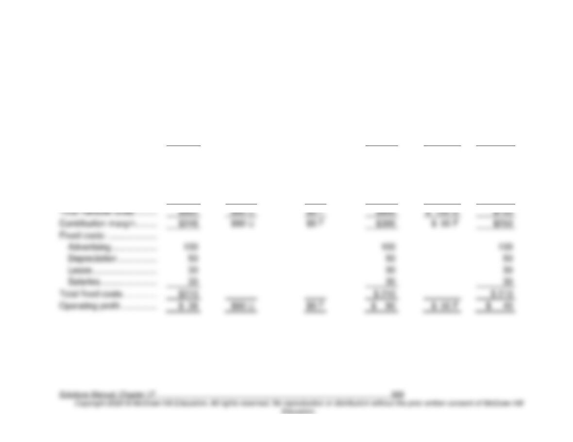
17–45. (40 min.) Analyze Performance for a Restaurant: Doug’s Diner.
Hint for working the problem: Use sales revenue as the basis for measuring volume.
($000)
Actual
Purchases
Variances
Marketing &
Administrative
Variances
Flexible
Budget
Activity
Variance
Master
Budget
Sales revenuea ……………
$1,200
$1,200
$200 F
$1,000
Variable costs:
Purchases………………..
780
$60 U
720
b
120 U
600
Hourly wages ……………
60
60
c
10 U
50
Franchise fee ……………
36
36
d
6 U
30
Utilities …………………….
76
$8 F
84
e
14 U
70
Total variable costs ………
$60 U
$8 F
$ 150 U
Contribution margin ………
$60 U
$8 F
$ 50 F
Fixed costs: ………………..
Advertising ……………….
100
100
100
50
Lease ………………………
30
30
30
Salaries……………………
30
30
30
Total fixed costs …………..
Notes on the following page.
17–45. (continued)
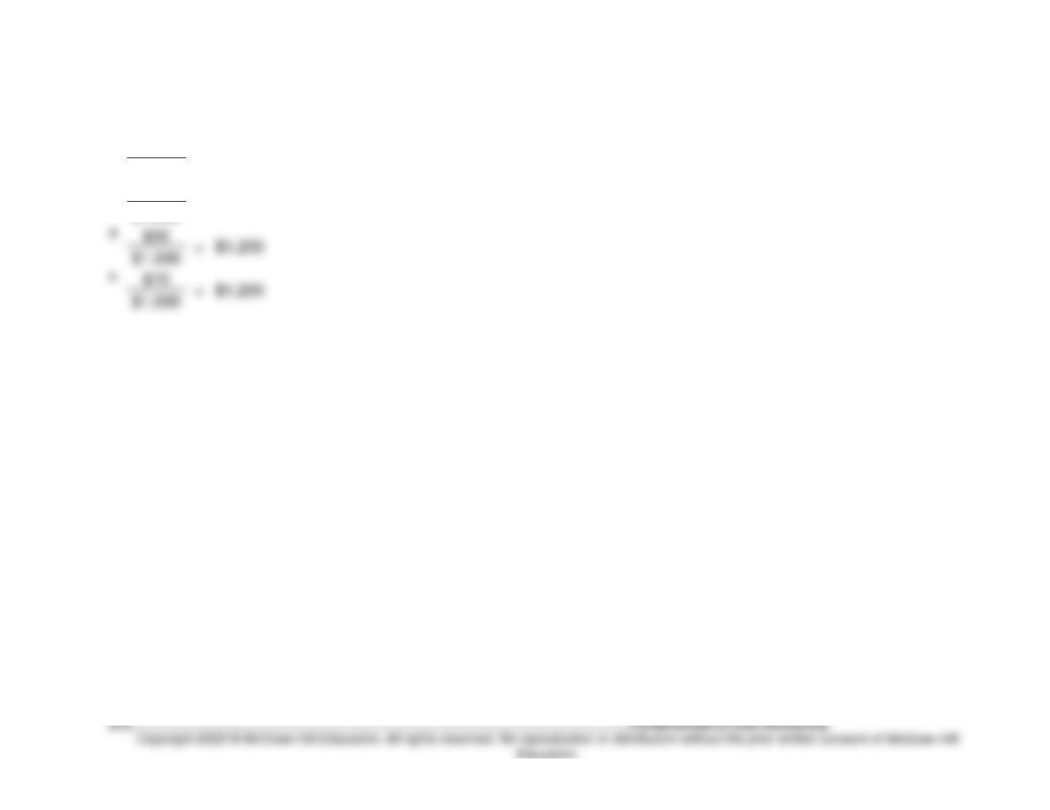
a Sales revenue is used as the basis of volume measurement because there are no price changes.
b
$600
×
$1,200
$1,000
c
$50
×
$1,200
$1,000
d
$30
e
17–46. (30 min.) Nonmanufacturing Cost Variances: FSBCU.
Incidental office costs comprise the variable costs. Salaries and the fixed office costs are
all fixed. Variance analysis for the two classes of overhead is as follows:
Actual Costs
Combined
Price and
Efficiency
Variance
Flexible Budget
(Standard Allowed for
Actual Output)
Correspondence,
Supplies, etc.
$17,280 × 0.95
= $16,416
$45 × 384
= $17,280
$864 F
Optional:
If computed, the production volume variance would be:
a 0.5 represents one-half year.
17–47. (30 min.) Performance Evaluation In Service Industries: Bay Area Bank.
Actual
Costs
Price
Variance
Actual
Inputs at
Standard
Price
Efficiency
Variance
Flexible
Budget
Activity
Variance
Master
Budget
New
Accounts
$572,250
(Ignored)
$30 ×
19,200
accounts
=
$576,000
$30 ×
20,000
accounts
=
$600,000
$3,750 F
$24,000 F
$2,550 F
17–48. (10 min.) Investigating Variances: Bay Area Bank.
Answers will vary. From the variance analysis above, it would be useful to better