17
Additional Topics in Variance Analysis
Solutions to Review Questions
17–1.
When production is not equal to sales, a portion of the sales comes from inventory or a
portion of production goes into inventory. In this case, the production costs expensed will
(generally) not be the same as the production costs incurred. In addition, a decision needs
to be made about whether to expense the entire variance or to prorate it between Cost of
Goods Sold and Finished Goods Inventory.
17–2.
False. Variances simply represent differences between plans and actual outcomes.
Capturing these variances can provide useful information regardless of whether
inventories exist. Knowledge about differences between plans and actual outcomes can
help managers improve planning or take steps to improve operations.
17–3.
Variances are usually “expensed” as a period cost (e.g., charged to Cost of Goods Sold).
17–4.
17–5.
17–6.
Some possible decisions for which the market share variance would be useful include
marketing (advertising) decisions, investment decisions, and product line portfolio
decisions.
17–7.
False. If a company has two or more products, a mix variance can arise even if the net
effect of all variances is zero. It might be very useful to learn about the mix variance
17–8.
Examples include:
17–9.
The concept of management by exception suggests managers not focus on things that are
proceeding according to plan. This allows time to focus on deviations (variances) from
expectations.
Solutions to Critical Analysis and Discussion Questions
17–10.
By recognizing the materials price variance at the time of purchase, management
captures any difference between actual materials cost and the standard costs as reflected
in the budget as those costs are incurred. If the price variance is not reflected until the
time of use, the effect of price changes might not be recognized until the materials are
removed from the raw materials inventory and placed into work in process. This could be
a substantial time delay. If decisions need to be made to compensate for the effect of
materials price changes, it would seem that the sooner the information comes to
management’s attention, the better the opportunities to react to the information.
17–11.
17–12.
In this situation the company is really selling just one product so a mix variance would not
be meaningful.
17–13.
In a hospital, as in other professional firms, billing rates vary with the level of the
17–14.
Salary rates vary according to the classification of the service providers (e.g., nurses’ pay
is higher than nurse practitioners’ pay), and the hospital will budget a certain amount of
time for each classification. Thus, a labor mix variance can be calculated to show if the
appropriate personnel were used in a particular period or in a particular unit (e.g.,
intensive care). An unfavorable mix variance would suggest that nurses were doing work
that nurse practitioners should have done.
17–15.
Disagree. The purpose of variance analysis is to identify items that are different from what
17–16.
Answers will vary. Variance analysis is helpful in any setting where budgets are
calculated, including business schools (and other academic institutions). In addition to the
usual price and volume variances, a sales mix variance will often be helpful, because
17–17.
Answers will vary. A company such as Uber with several services (Uber-X, Uber-Black,
and so on), would likely learn something from sales activity and mix. Whether they would
Solutions to Exercises
17–18. (25 min.) Prorating Direct Labor Cost Variances: Cook Company.
a. and b. Direct labor variances:
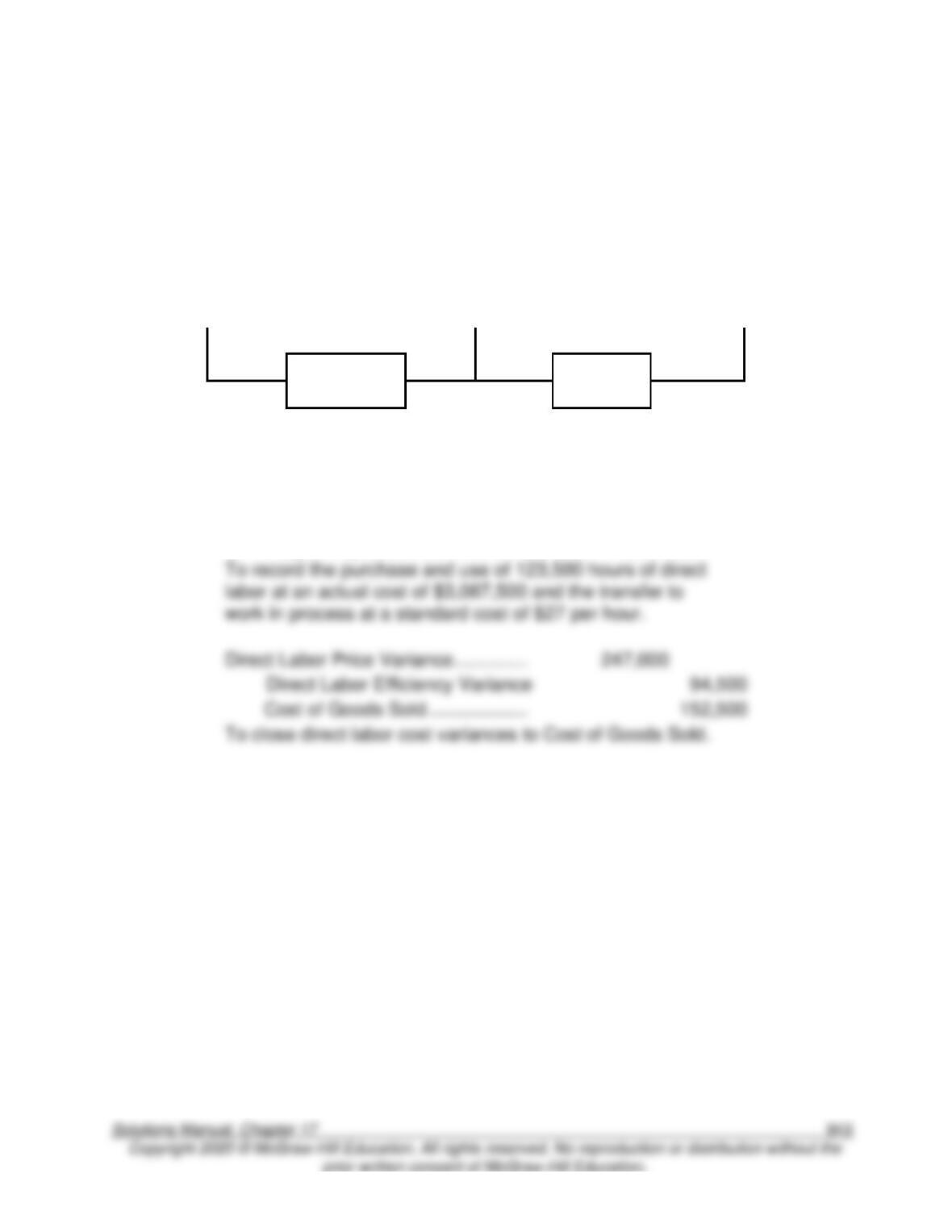
$3,087,500
$27.00 × 123,500
= $3,334,500
$27.00 × 2 hrs ×
60,000
= $3,240,000
$247,000 F
$94,500 U
c.
Work-in-Process Inventory ………..
3,240,000
Direct Labor Efficiency Variance …
94,500
Direct Labor Price Variance ..
247,000
Wages Payable …………………
3,087,500
Direct Labor Price Variance …………..
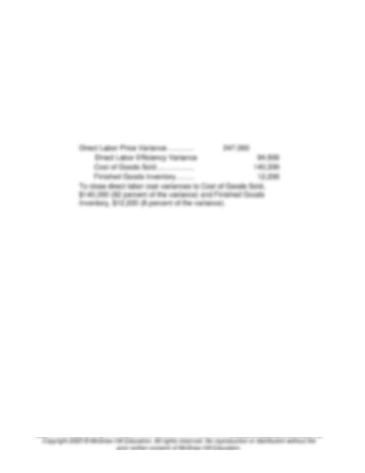
Direct Labor Efficiency Variance
To close direct labor cost variances to Cost of Goods Sold.
17-18 (continued)
d.
Finished Goods Inventory is 8 percent (= 4,800 ÷ 60,000) of production).
Work-in-Process Inventory ………..
3,240,000
Direct Labor Efficiency Variance ..
94,500
Direct Labor Price Variance .
247,000
Wages Payable ………………..
3,087,500
To record the purchase and use of 123,500 hours of direct
labor at an actual cost of $3,087,500 and the transfer to
work in process at a standard cost of $27 per hour.
Direct Labor Price Variance ………….
Direct Labor Efficiency Variance
Cost of Goods Sold……………….
Finished Goods Inventory ………
To close direct labor cost variances to Cost of Goods Sold,
$140,300 (92 percent of the variance) and Finished Goods
Inventory, $12,200 (8 percent of the variance).
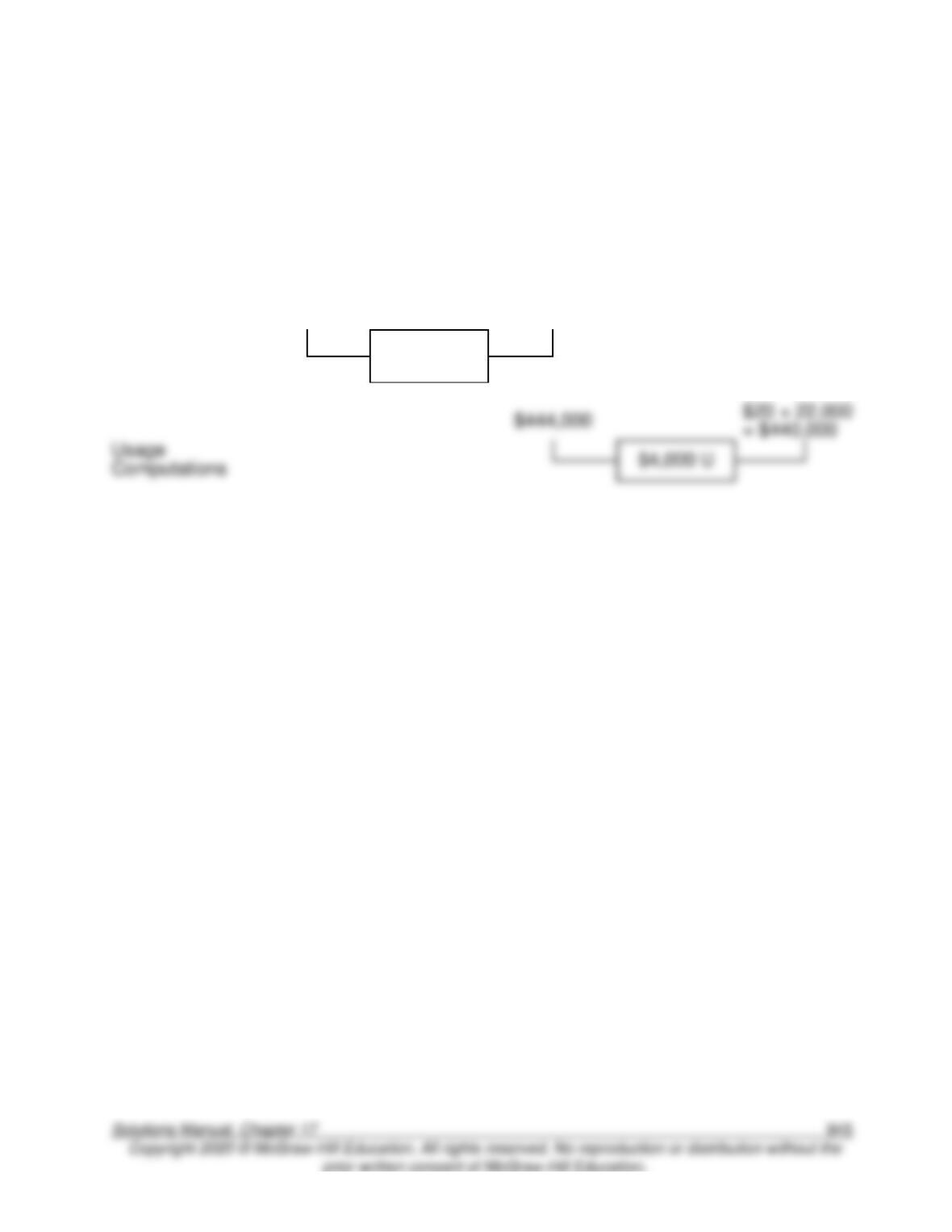
17–19. (15 min.) Variable Cost Variances: Materials Purchased And Materials Used
Are Not Equal: Gates Corporation.
Actual
Costs
Price
Variance
Actual
Inputs at
Standard
Price
Efficiency
Variance
Flexible
Budget
(Standard
Allowed for
Good Output)
Purchase
Computations
$673,000
$688,000
$15,000 F
= $440,000
17–20. (15 min.) Prorating Direct Materials Variances: Gates Corporation.
a.
Work-in-Process Inventory ………..
440,000
Direct Materials Efficiency Variance
4,000
Direct Materials Inventory …..
444,000
To record the standard cost of materials used and the
materials efficiency variance.
Direct Materials Inventory …………….
Direct Materials Price Variance
Accounts Payable …………………
Direct Materials Price Variance ……..
15,000
Direct Materials Efficiency Variance
4,000
Cost of Goods Sold……………….
11,000
To close direct labor cost variances to Cost of Goods Sold.
b.
Finished Goods Inventory is 1/11 (= 2,000 ÷ 22,000) of production.
Work-in-Process Inventory ………..
440,000
Direct Materials Efficiency Variance
4,000
Direct Materials Inventory …..
444,000
To record the standard cost of materials used and the
materials efficiency variance.
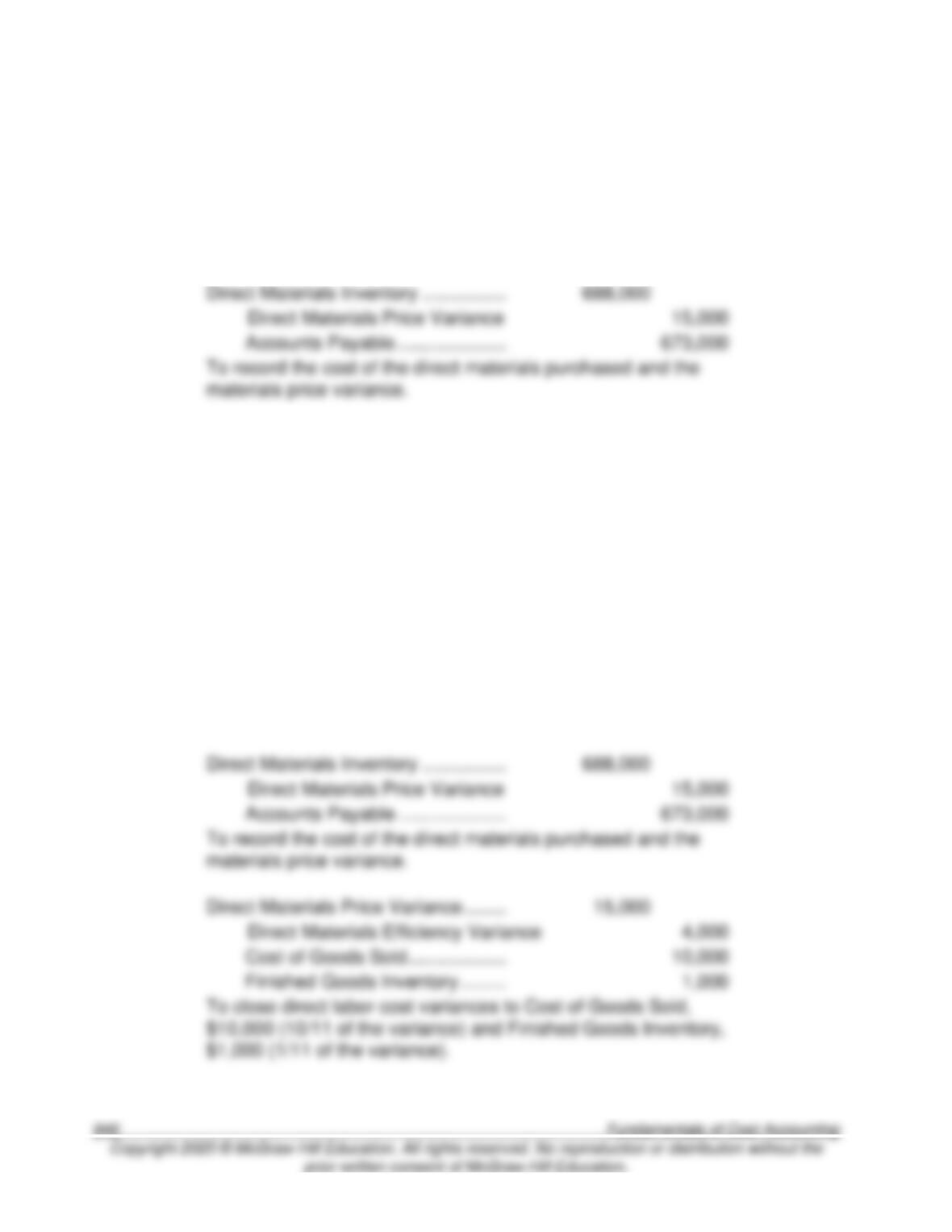
Direct Materials Inventory …………….
Direct Materials Price Variance
Accounts Payable …………………
To record the cost of the direct materials purchased and the
materials price variance.
Direct Materials Price Variance ……..
Direct Materials Efficiency Variance
Cost of Goods Sold……………….
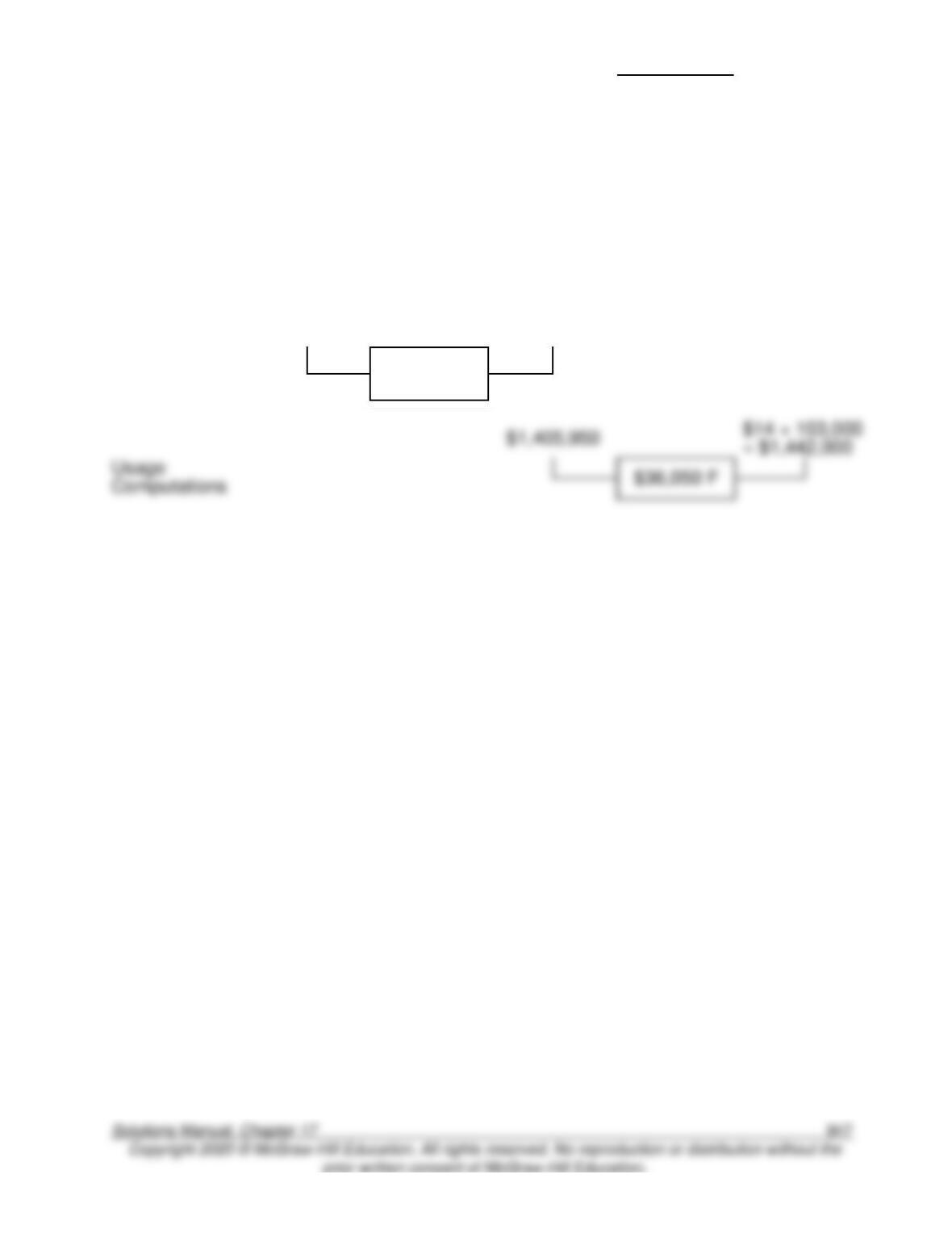
17–21. (15. Min) Variable Cost Variances: Materials Purchased And Used Are Not
Equal: Mathis, Inc.
Actual
Costs
Price
Variance
Actual
Inputs at
Standard
Price
Efficiency
Variance
Flexible
Budget
(Standard
Allowed for
Good Output)
Purchase
Computations
$1,642,800
$1,554,000
$88,800 U
= $1,442,000
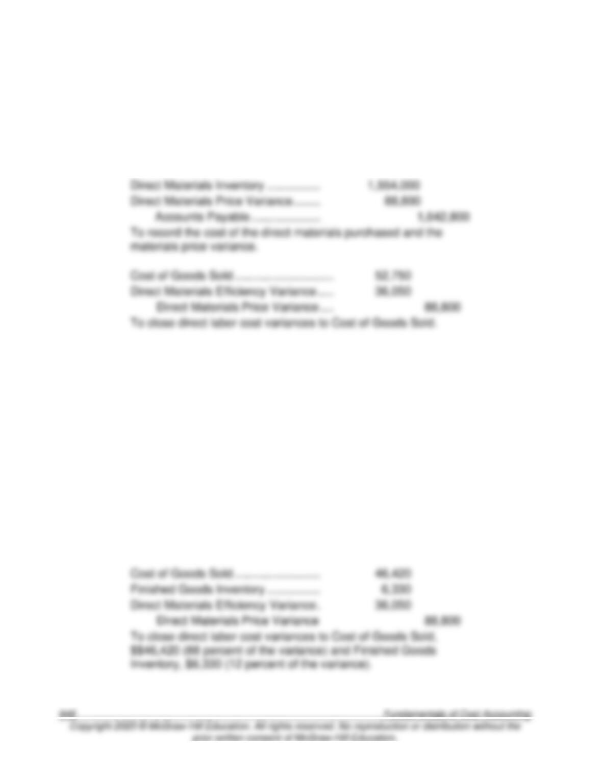
17–22. (15 min.) Prorating Direct Materials Variances: Mathis, Inc.
a.
Work-in-Process Inventory ……………….
1,442,000
Direct Materials Efficiency Variance
36,050
Direct Materials Inventory ………….
1,405,950
To record the standard cost of materials used and the materials
efficiency variance.
Direct Materials Inventory …………….
Direct Materials Price Variance ……..
Accounts Payable …………………
1,642,800
Cost of Goods Sold …………………………
Direct Materials Efficiency Variance …..
Direct Materials Price Variance ….
To close direct labor cost variances to Cost of Goods Sold.
b.
Units sold are 88 percent (= 90,640 ÷ 103,000) of production.
Work-in-Process Inventory ……………….
1,442,000
Direct Materials Efficiency Variance
36,050
Direct Materials Inventory ………….
1,405,950
To record the standard cost of materials used and the materials
efficiency variance.
Direct Materials Inventory …………….
1,554,000
Direct Materials Price Variance ……..
88,800
Accounts Payable …………………
1,642,800
To record the cost of the direct materials purchased and the
materials price variance.
Cost of Goods Sold ……………………..
Finished Goods Inventory …………….
Direct Materials Efficiency Variance .
Direct Materials Price Variance
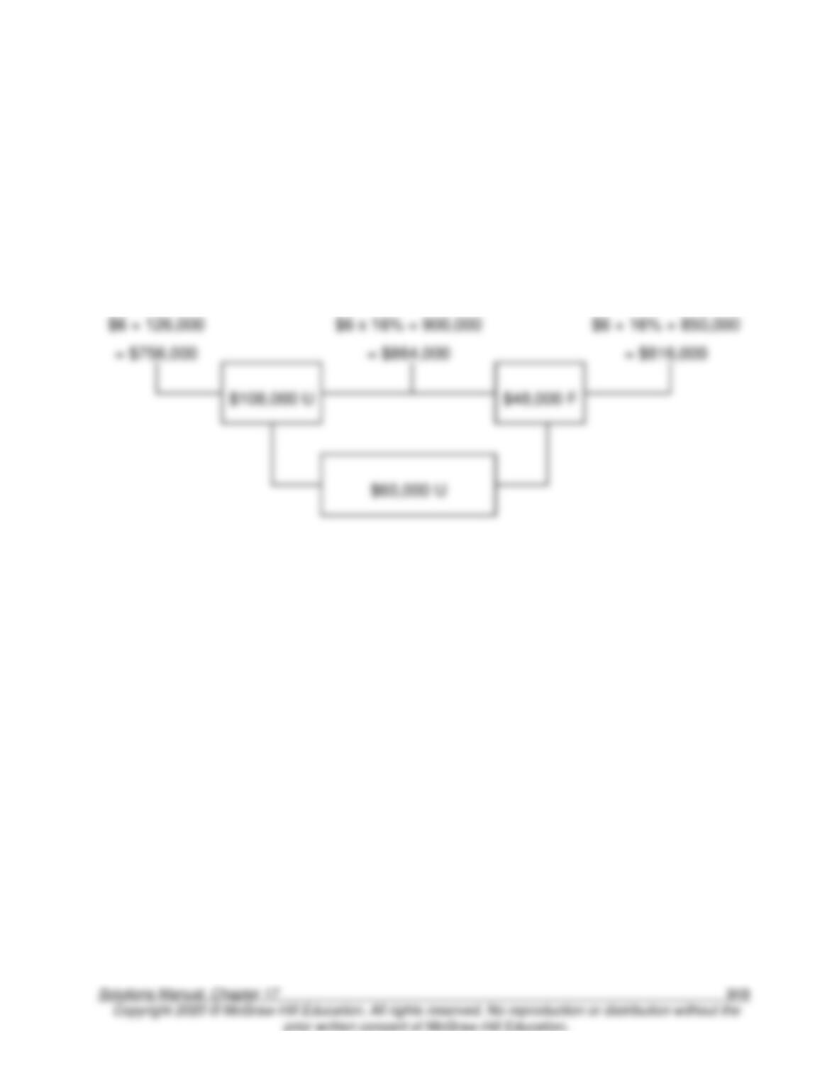
17–23. (15 min.) Industry Volume and Market Share Variances: D&B Ice Cream.
Flexible Budget
(SCM × AQ)
Market
Share
Variance
Standard
Contribution Margin
Times Budgeted
Market Share Times
Actual Industry
Volume
(SCM × ASQ)
Industry
Volume
Variance
Master Budget
(SCM × SQ)
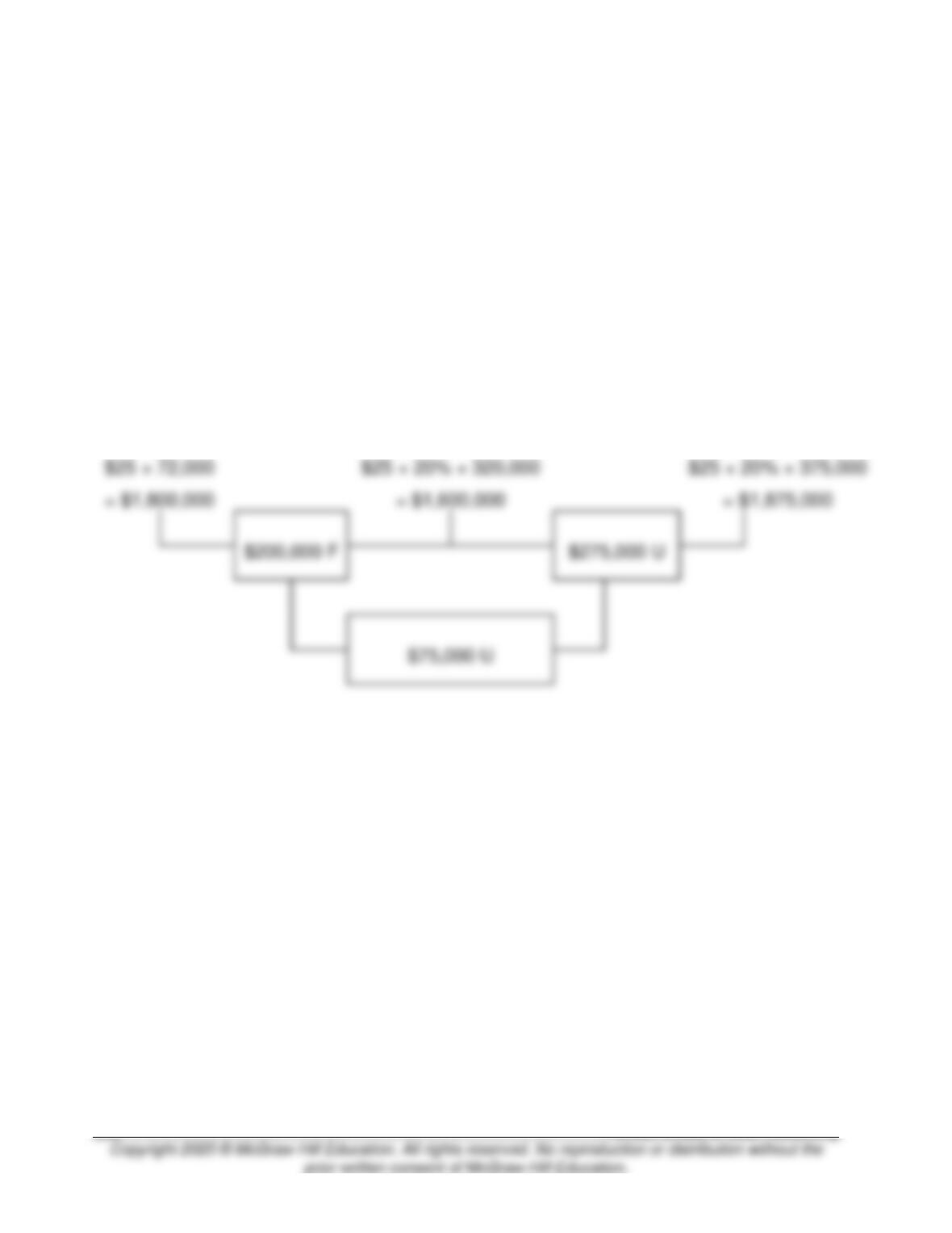
17–24. (15 min.) Industry Volume and Market Share Variances: Olive Tree Products.
The budgeted contribution margin is $25 (= $45 – $20). (Note that the fixed costs are
irrelevant in this exercise.)
The budgeted industry volume was 375,000 units (75,000 units ÷ 20%).
Flexible Budget
(SCM × AQ)
Market
Share
Variance
Standard Contribution
Margin Times
Budgeted Market
Share Times Actual
Industry Volume
(SCM × ASQ)
Industry
Volume
Variance
Master Budget
(SCM × SQ)
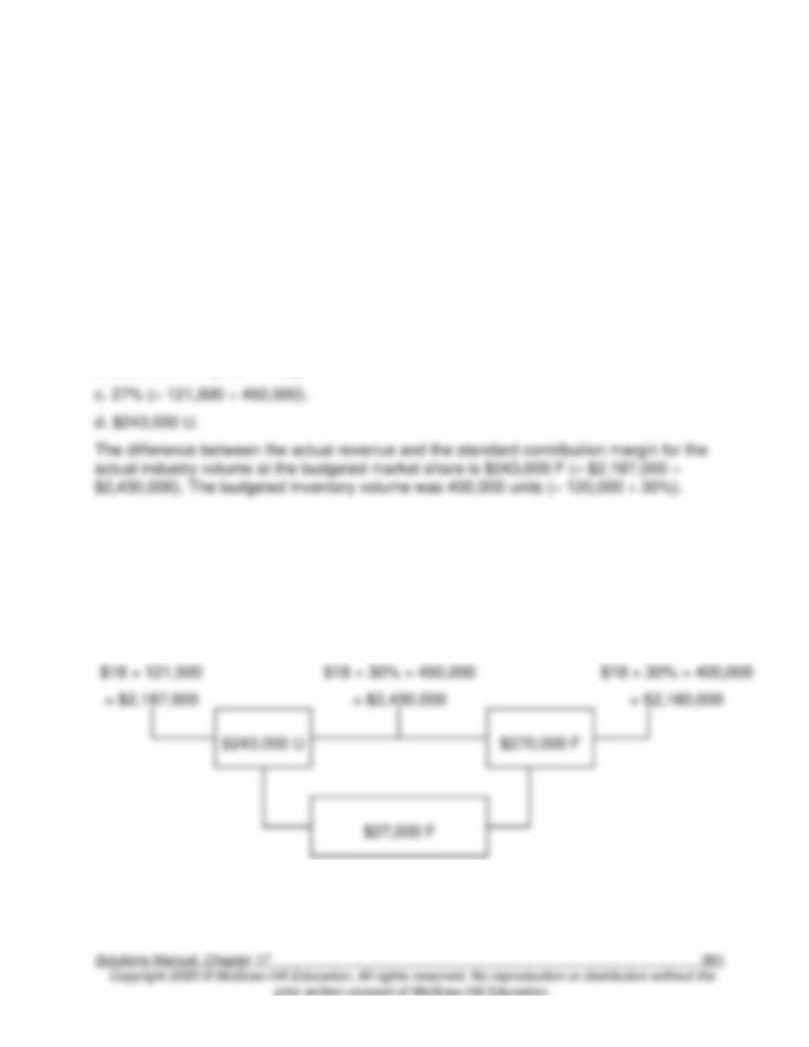
17–25. (15 min.) Industry Volume and Market Share Variances: Albury Corporation.
a. $18 per unit.
The sales activity variance is:
Budgeted contribution margin per unit (BCM) × (Actual Sales – Budgeted Sales).
So,
BCM = $18 = $27,000 ÷ (121,500 – 120,000).
b. 450,000 units.
The master budget contribution margin is $2,160,000 (= $18 × 120,000). The industry
volume variance is $270,000 F, so the standard contribution margin for the actual industry
volume at the budgeted market share is $2,430,000 (= $2,160,000 + $270,000). Given the
budgeted contribution margin per unit of $18, the actual industry volume is 450,000 units
[= $2,430,000 ÷ ($18 × 30%)].
Flexible Budget
(SCM × AQ)
Market
Share
Variance
Standard Contribution
Margin Times
Budgeted Market
Share Times Actual
Industry Volume
(SCM × ASQ)
Industry
Volume
Variance
Master Budget
(SCM × SQ)
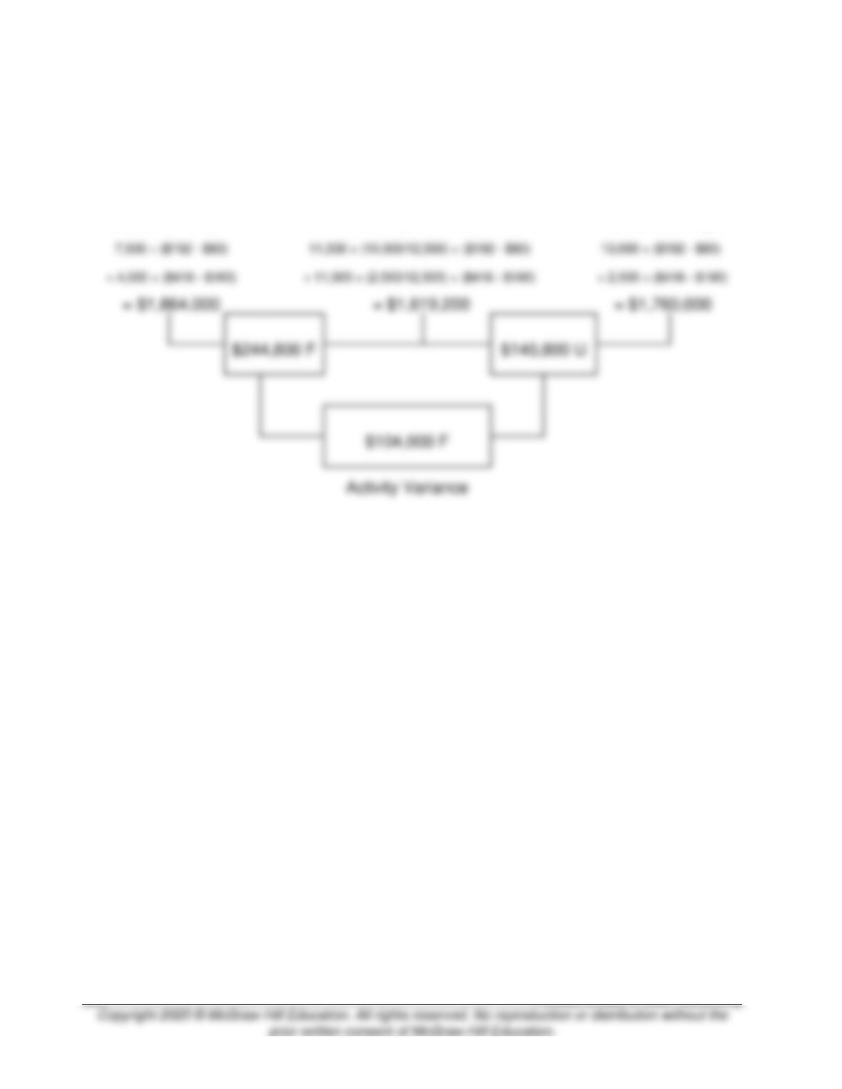
17–26. (20 min.) Sales Mix and Quantity Variances: A-Zone Media.
a. and b.
The actual prices are not relevant here. The mix and quantity variances are based on
standard (budgeted) contribution margin per unit.
Flexible Budget
AQ × (SP – SV)
Mix
Variance
ASQ × (SP – SV)
Quantity
Variance
Master Budget
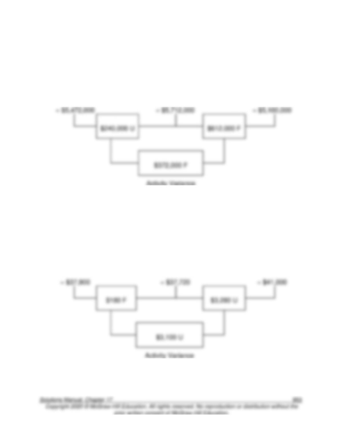
17–27. (20 min.) Sales Mix and Quantity Variances: Sara’s Systems.
a. and b.
Flexible Budget
AQ × (SP – SV)
Mix
Variance
ASQ × (SP – SV)
Quantity
Variance
Master Budget
26,400 × ($200 – $80)
+ 7,200 × ($480 – $160)
33,600 × (22,500/30,000) × ($200 – $80)
+ 33,600 × (7,500/30,000) × ($480 – $160)
22,500 × ($200 – $80)
+ 7,500 × ($480 – $160)
Activity Variance
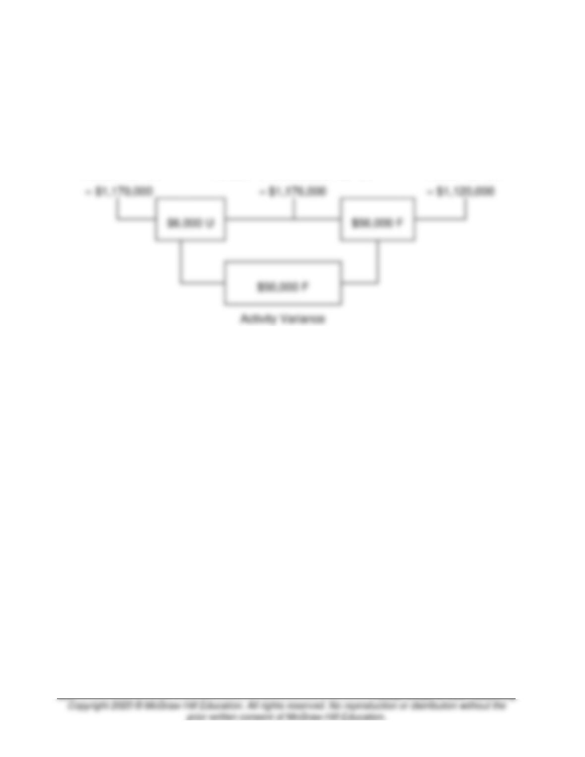
17–28. (20 min.) Sales Mix and Quantity Variances: Hotel Galaxy.
a. and b.
Flexible Budget
AQ × (SP – SV)
Mix
Variance
ASQ × (SP – SV)
Quantity
Variance
Master Budget
950 × ($35 – $15)
+ 1,350 × ($24 – $10)
2,300 × (1,000/2,500) × ($35 – $15)
+ 2,300 × (1,500/2,500) × ($24 – $10)
1,000 × ($35 – $15)
+ 1,500 × ($24 – $10)
17–29. (20 min.) Sales Mix and Quantity Variances: Chow-4-Hounds.
a. and b.
Flexible Budget
AQ × (SP – SV)
Mix
Variance
ASQ × (SP – SV)
Quantity
Variance
Master Budget
60,000 × ($12 – $5)
+ 150,000 × ($9 – $4)
210,000 × (60,000/200,000) × ($12 – $5)
+ 210,000 × (140,000/200,000) × ($9 – $4)
60,000 × ($12 – $5)
+ 140,000 × ($9 – $4)
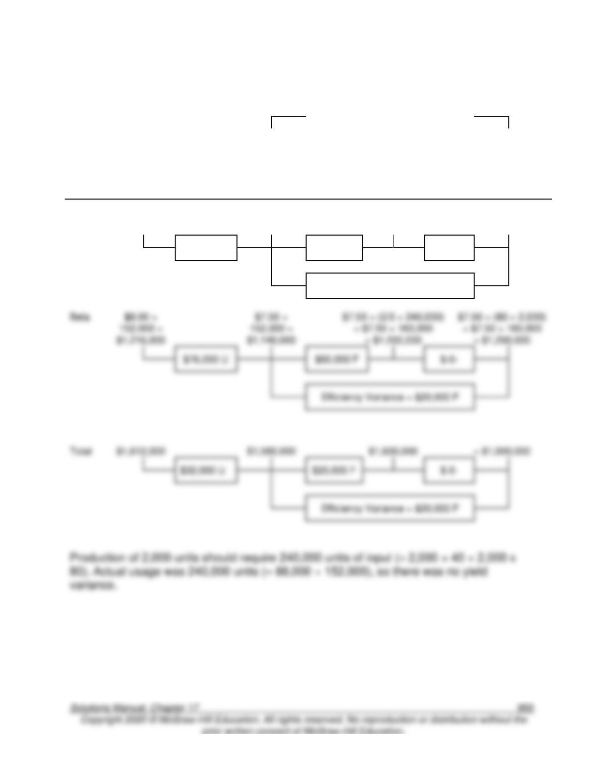
17–30. (35 min.) Materials Mix and Yield Variances: Stacy, Inc.
a. and b.
Efficiency Variance
Actual
(AP × AQ)
Purchase
Price
Variance
(SP × AQ)
Mix
Variance
(SP × ASQ)
Yield
Variance
Flexible
Production
Budget (SP ×
SQ)
Material:
Alpha
$4.50 ×
88,000 =
$396,000
$5.00 ×
88,000 =
$440,000
$5 × (1/3 × 240,000) =
$5.00 × 80,000
= $400,000
$5 × (40 × 2,000) =
$5 × 80,000 =
$400,000
$44,000 F
$40,000 U
$-0-
Efficiency Variance = $40,000 U
Beta
$7.50 ×
152,000 =
= $1,200,000
= $7.50 × 160,000
$-0-
Total
$-0-
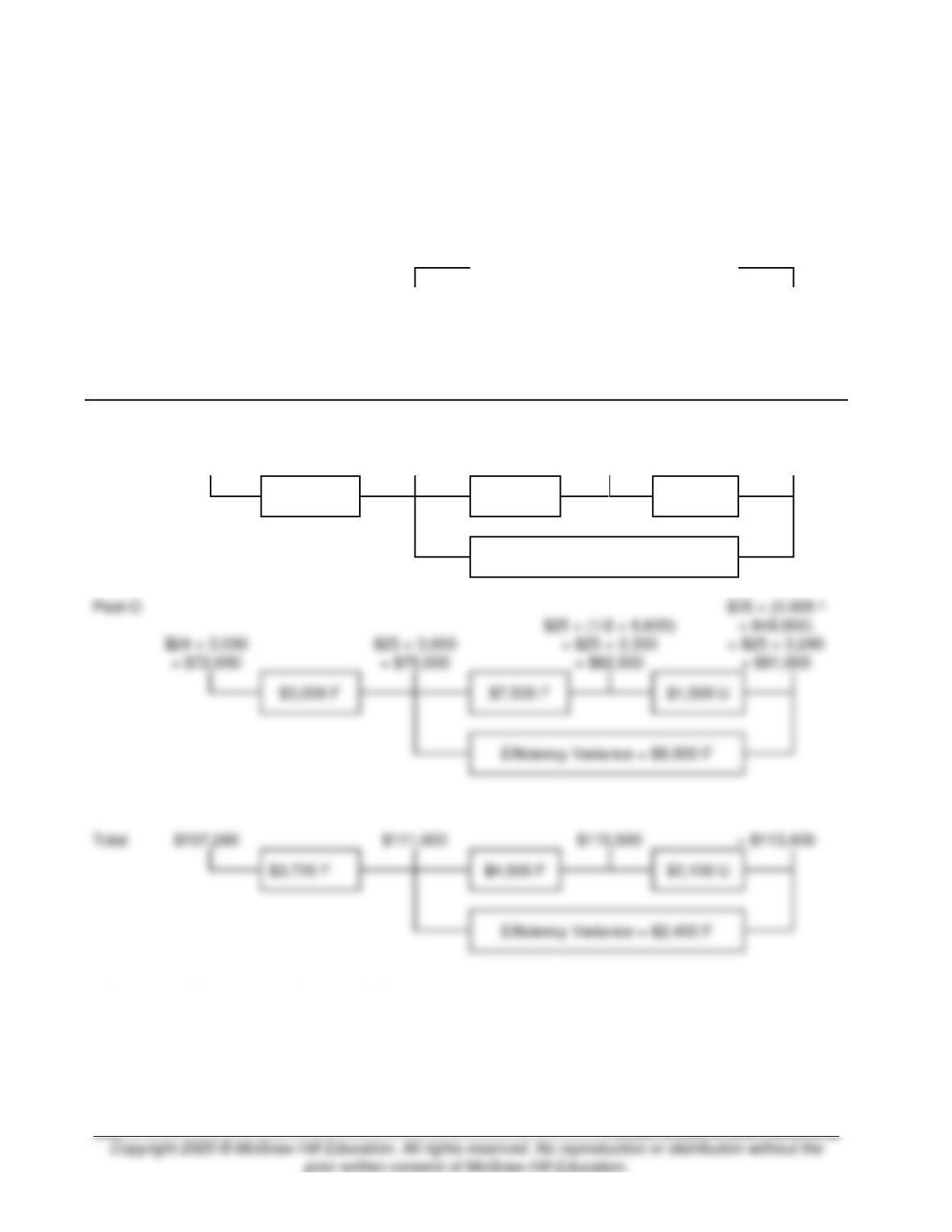
17–31. (35 min.) Materials Mix and Yield Variances: John’s Weed-B-Gone.
a. and b.
The actual purchase prices were $9.80 (= $35,280 ÷ 3,600) for Weed-X and $24.00 (=
$72,000 ÷ 3,000) for Pest–O.
Efficiency Variance
Actual
(AP × AQ)
Purchase
Price
Variance
(SP × AQ)
Mix
Variance
(SP × ASQ)
Yield
Variance
Flexible
Production
Budget
(SP × SQ)
Material:
Weed-X
$9.80 ×
3,600
= $35,280
$10 × 3,600
= $36,000
$10 × (1/2 × 6,600)
= $10 × 3,300
= $33,000
$10 × (0.005 a
× 648,000)
= $10 × 3,240
= $32,400
$720 F
$3,000 U
$600 U
Efficiency Variance = $3,600 U
$3,000 F
Total
$107,280
$2,100 U
a (1 gallon ÷ 100 square yards) ÷ 2 = 0.005
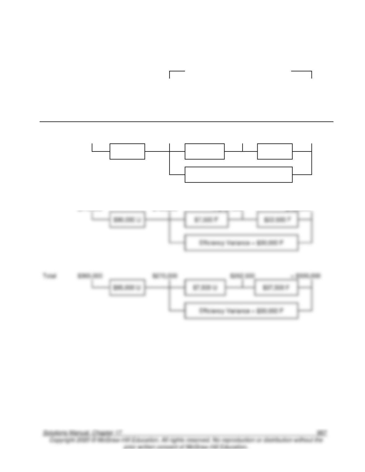
17–32. (35 min.) Labor Mix and Yield Variance: Matt’s Eat ‘N Run.
a. and b.
Efficiency Variance
Actual
(AP ×
AQ)
Purchase
Price
Variance
(SP × AQ)
Mix
Variance
(SP ×
ASQ)
Yield
Variance
Flexible
Production
Budget
(SP × SQ)
Labor:
Skilled
$125,000
$20 × 6,000
= $120,000
$20 × (0.25 × 21,000)
= $20 × 5,250
= $105,000
$20 × (2/60 × 180,000)
= $20 × 6,000
= $120,000
$5,000 U
$15,000 U
$15,000 F
Efficiency Variance = $-0-
Unskilled
$240,000
Total
$365,000
$270,000
$10 ×
15,000 =
$10 × (0.75 × 21,000)
= $10 × 15,750
$10 × (6/60 × 180,000)
= $10 × 18,000 =
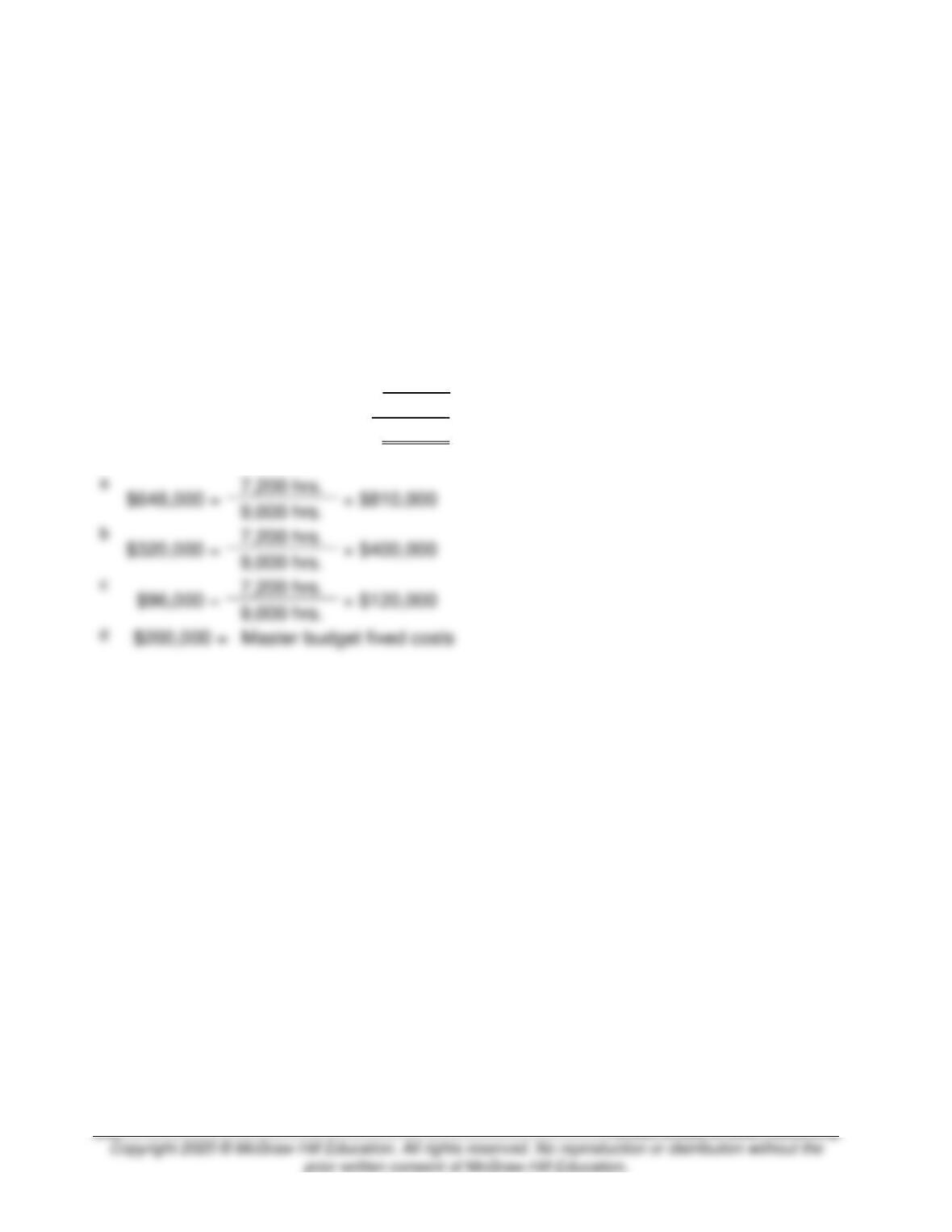
17–33. (10 min.) Flexible Budgeting—Service Organization: K&B.
Flexible Budget
(based on
actual of
7,200 hours)
Revenue ………………………….
$648,000a
Costs:
Professional salaries ………
320,000b
Other variable costs ……….
96,000c
Fixed costs ……………………
200,000d
Total costs …………………
$616,000
Profit ……………………………….
$32,000