
CHAPTER 16
COST-VOLUME-PROFIT ANALYSIS
Cost-volume-profit (CVP) analysis can be used to illustrate how managers use accounting data for
planning and decision making. Students who enjoy solving puzzles will probably enjoy the discussion of
CVP. A more complete analysis of the subject material can be taught by using simple algebra.
LEARNING OBJECTIVES
After studying Chapter 16, students should be able to:
1. Determine the number of units and amount of sales revenue needed to break even and to earn a target
profit.
2. Determine the number of units and sales revenue needed to earn an after-tax target profit.
3. Apply cost-volume-profit analysis in a multiple-product setting.
4. Prepare a profit-volume graph and a cost-volume-profit graph, and explain the meaning of each.
5. Explain the impact of risk, uncertainty, and changing variables on cost-volume-profit analysis.
6. Discuss the impact of non-unit cost drivers on cost-volume-profit analysis.
KEY TOPICS
The following major topics are covered in this chapter (related learning objectives are listed for each
topic):
1. The Break-Even Point and Target Profit in Units and Sales Revenue (LO 1)
2. After-Tax Profit Targets (LO 2)
3. Multiple-Product Analysis (LO 3)
4. Graphical Representation of CVP Relationships (LO 4)
5. Changes in the CVP Variables (LO 5)
6. CVP Analysis and Non-Unit Cost Drivers (LO 6)
I. THE BREAK-EVEN POINT AND TARGET PROFIT IN UNITS AND SALES REVENUE
To find out how revenues, expenses, and profits behave as volume changes, it is natural to begin by
finding the firm’s break-even point (the point of zero profit) in units sold and in sales revenue. Two
frequently used approaches to finding the break-even point are the operating income approach and the

contribution margin approach. Operating income is income or profit before income taxes. Contribution
margin is sales revenue minus total variable costs.
The operating income approach uses the following basic equation:
Operating income = Sales revenue – Variable expenses – Fixed expenses
Sales revenue is equal to the unit selling price times the number of units sold. Total variable costs equal
the unit variable cost times the number of units sold. Therefore, the operating income equation can also be
expressed as follows:
Operating income = (Price × Number of units) – (Variable cost per unit ×
Number of units) – Total fixed costs
Finally, the equation for a target profit is put in terms of units:
Units for a target profit = (Total fixed cost + Target income)/(Price – Variable cost per unit)
Cornerstone 16.2 (p. 827) shows how and why to calculate the units needed to break even and to achieve
a target profit.
By substituting the unit contribution margin for price minus unit variable cost in the operating income
equation, and solving for the number of units, the following break-even expression is obtained:
Number of units = Fixed costs/Unit contribution margin
To calculate the break-even point in sales revenue, variable costs are defined as a percentage of sales
rather than as an annual per unit sold. To express variable cost in terms of sales revenue, we compute the
variable cost ratio, which is the proportion of each sales dollar that must be used to cover variable costs.
The percentage of sales revenue remaining after variable costs are covered is the contribution margin
ratio. The contribution margin ratio is the proportion of each sales dollar available to cover fixed costs
and provide for profit.
The sales-revenue approach is computed by using the following equation:
Sales = (Total fixed costs + Operating income)/Contribution margin ratio
At break-even, operating income equals zero, so the equation becomes:
Break-even sales = Total fixed costs/Contribution margin ratio
Cornerstone 16.3 (p. 831) illustrates the calculation of break-even sales revenue and sales revenue needed
to achieve a target profit for Blazin-Boards Company.
II. AFTER-TAX PROFIT TARGETS
To determine the number of units that must be sold to reach an after-tax profit target, first convert the
after-tax profit to a before-tax profit target. To do this, divide the after-tax profit by (1 − Tax rate). Then,
the desired before-tax profit can be used in the target profit formula presented on the following page.
Operating income = Net income/(1 – Tax rate)
Cornerstone 16.4 (p. 833) shows how to calculate the number of units needed to achieve an after-tax
profit target.
Teaching hint: At this point in the discussion, you may wish to use the following example:
Fixed costs
$40,000
Selling price per unit
$10
Variable cost per unit
$6
Tax rate
40%
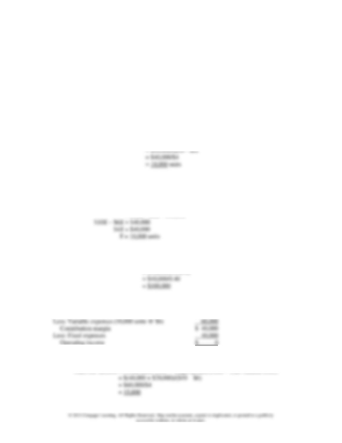
1. What is the break-even point in units?
Number of units = Fixed costs/(Price – Unit variable cost)
The break-even point in units can also be found as follows:
Let X = break-even point in units.
Operating income = Sales revenues − Variable expenses − Fixed expenses
= $10X − $6X − $40,000
2. What is the break-even point in dollars?
Break-even sales = Total fixed costs/Contribution margin ratio
= $40,000/($4/$10)
3. Prepare an income statement for the break-even level.
Sales (10,000 units @ $10)
$100,000
Less: Variable expenses (10,000 units @ $6)
Contribution margin
Less: Fixed expenses
40,000
Operating income
4. How many units must be sold to obtain a targeted profit before taxes of $20,000?
Units for $20,000 = (Total fixed costs + Target profit)/(Price – Unit variable costs)
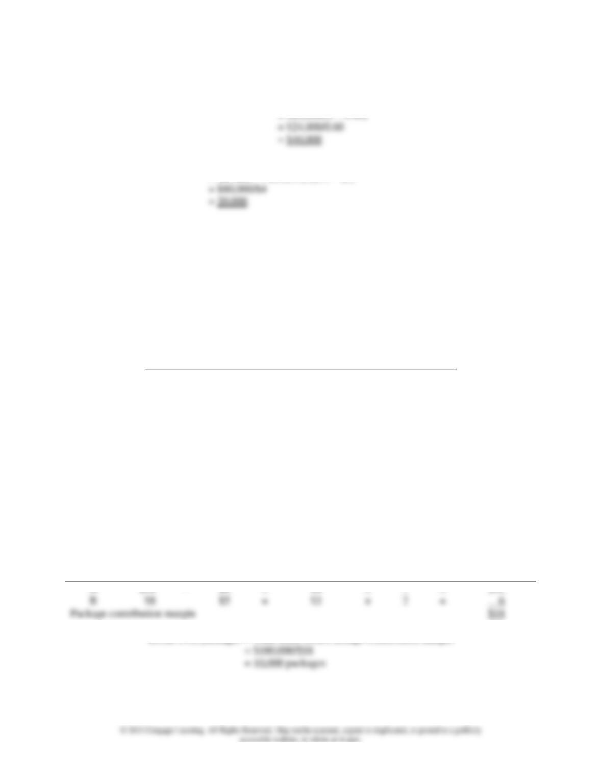
5. How many units must be sold to obtain a targeted profit after taxes of $24,000?
Before-tax income = After-tax income/(1 – Tax rate)
Units for $24,000 = (Total fixed costs + Target profit)/(Price – Unit variable costs)
= ($40,000 + $40,000)/($10 – $6)
III. MULTIPLE-PRODUCT ANALYSIS
To determine the break-even point in units for multiple products, you must convert the multiple-product
problem into a single-product problem. The key to this conversion is to identify the expected sales mix.
Sales mix is the relative combination of products being sold by a firm. It can be measured in units sold or
in proportion of revenue.
Teaching hint: The following example can be put on the board to study multiple-product analysis:
Product
Sales Mix
Price
Unit Variable
Cost
A
3
$10
$6
B
2
8
5
Total fixed expenses = $180,000
Ask the students how many units of A and how many units of B must be sold to break even. It shouldn’t
take them long to realize that the problem is more complicated than the single-product setting. Explain
that the methodology developed for CVP analysis is for a single-product setting. To apply this
methodology, we must convert the multiple-product problem into a single-product problem. Ask your
students how this might be done. Usually, someone will suggest defining the single product as the mix
consisting of three units of A and two units of B.
The solution follows:
Product
Price
–
Unit
Variable
Cost
=
Unit
Contribution
Margin
×
Sales
Mix
=
Total
Contribution
Margin
A
$10
–
$6
=
$4
×
3
=
$12
$8
$5
$3
6
Package contribution margin
$18
Break-even packages = Total fixed costs/Package contribution margin
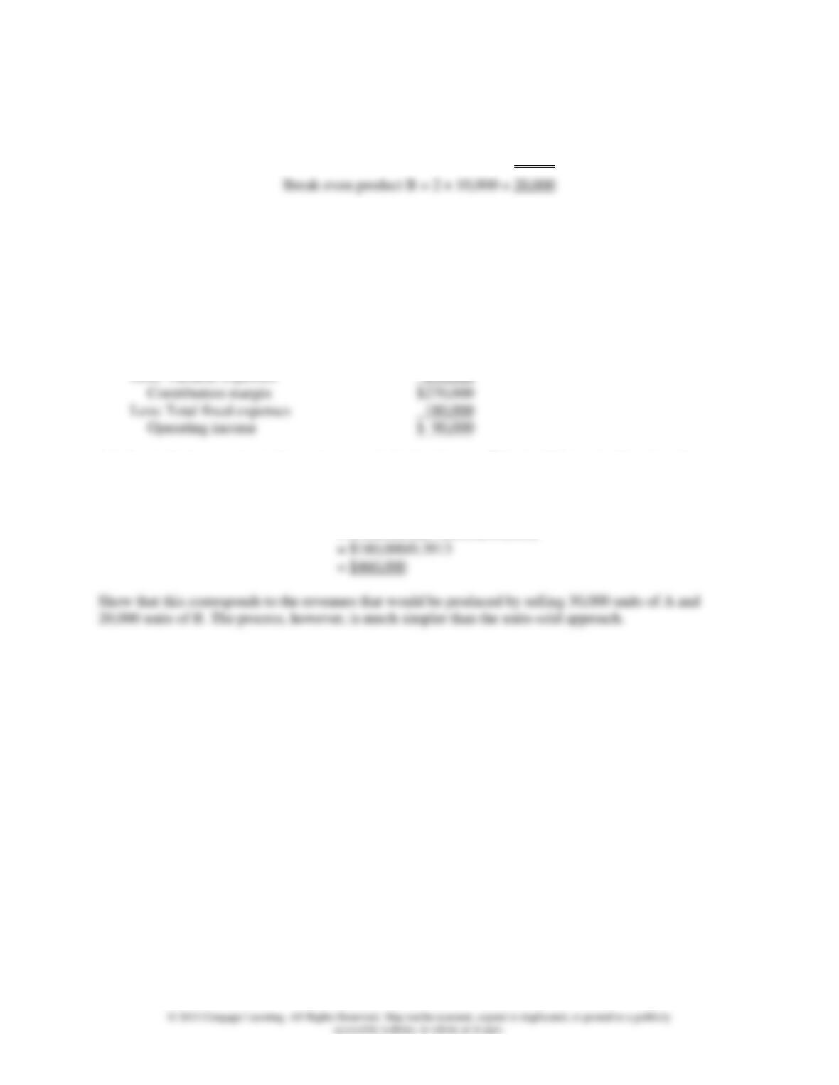
Each package contains 3 units of A and 2 units of B. Therefore, to break even, we need to sell the
following units of A and B:
Break-even product A = 3 × 10,000 = 30,000
Teaching hint: Some students worry that they won’t choose the “correct” sales mix numbers. You might
emphasize that it is the proportion that is important. Solve the above problem using a sales mix of 30
units of A and 20 units of B, or 6 units of A and 4 units of B, to show that the same break-even point is
reached.
To illustrate the utility of the sales-revenue approach, put the following income statement on the board,
and indicate that it corresponds to the statement associated with products A and B.
Sales
$690,000
Contribution margin
$270,000
Less: Total fixed expenses
180,000
Ask the students to compute the revenues needed to break even. This should be a simple task and most
should produce the following answer:
Break-even sales = Total fixed costs/Contribution margin ratio
= $180,000/($270,000/$690,000)
IV. GRAPHICAL REPRESENTATION OF CVP RELATIONSHIPS
A graphical representation can help managers see the difference between variable cost and revenue and
deepens their understanding of CVP relationships. It may also help managers understand quickly what
impact an increase or decrease in sales will have on the break-even point. Two basic graphs are presented
in the text: the profit-volume graph and the cost-volume-profit graph. A profit-volume graph portrays the
relationships between profits and sales volume. Exhibit 16.2 (p. 840) depicts a profit-volume graph for
Gordon Company. The cost-volume-profit graph depicts the relationships among cost, volume, and
profits. Exhibit 16.3 (p. 841) depicts a cost-volume-profit graph for Gordon Company.
Teaching hint: You may want to teach students about cost-volume-profit graphs by presenting a series of
graphs. First, put separate graphs on the board for total variable costs and total fixed costs. Then, combine
these graphs into a third graph and refer to it as a total cost curve. Now, introduce the total revenue graph.
Finally, combine the total cost and total revenue graphs into one graph and refer to it as the cost-volume-
profit graph. (See Exhibit 16.3 on page 841.)
A number of assumptions are commonly mentioned with respect to CVP analysis:
1. The analysis assumes a linear revenue function and a linear cost function.
2. The analysis assumes that price, total fixed costs, and unit variable costs can be accurately
V. CHANGES IN THE CVP VARIABLES
This section briefly discusses the margin of safety and operating leverage. The margin of safety is the
units sold or expected to be sold or the revenue earned or expected to be earned above the break-even
volume. Operating leverage is concerned with the relative mix of fixed and variable costs in an
organization. It is the use of fixed costs to extract higher percentage changes in profits as sales activity
changes. The greater the degree of operating leverage, the more that changes in sales activity will affect
profits. Because of this phenomenon, the mix of costs that an organization chooses can have a
considerable influence on its operating risk and profit level.
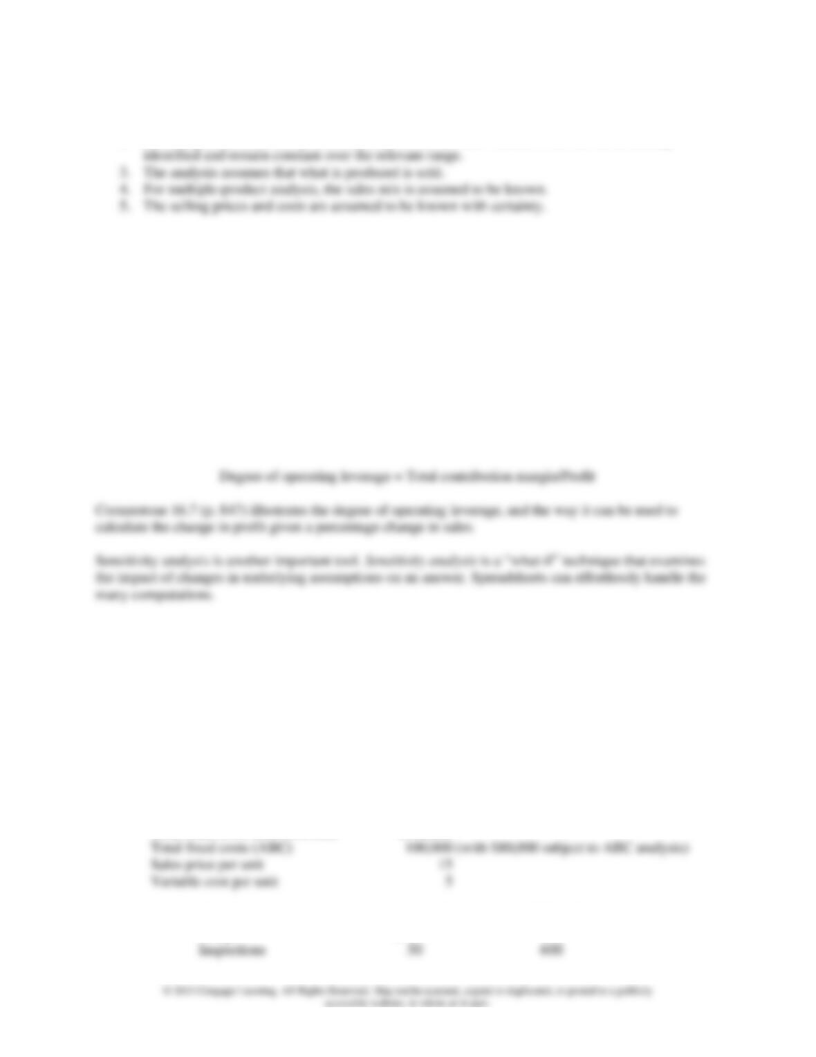
The degree of operating leverage can be measured for a given level of sales by taking the ratio of total
contribution margin to profit, as follows:
VI. CVP ANALYSIS AND NON-UNIT COST DRIVERS
Conventional CVP analysis assumes that all costs of the firm can be divided into two categories: those
that vary with sales volume (variable costs) and those that do not (fixed costs). Furthermore, costs are
assumed to be a linear function of sales volume. Frequently, however, there are costs that vary with non–
unit cost drivers. An activity-based costing (ABC) system, in which costs are divided into unit- and non-
unit-based categories, is a good example of this. The following example may help you to illustrate the
calculations.
Assume the following:
Total fixed costs (conventional)
$180,000
Total fixed costs (ABC)
Sales price per unit
15
Variable cost per unit
5
Cost Driver
Unit Variable Cost
Level of Cost Driver
Setups
$500
100
Inspections
50
1. What is the break-even point in units under conventional analysis?
Break-even units = Fixed costs/(Price – Unit variable cost)
= $180,000/($15 – $5)
2. What is the break-even point in units under ABC analysis?
Break-even units = [Fixed costs + (Setup cost × Number of setups) + (Inspection cost × Number of
inspections)]/(Price – Unit variable cost)
= [$100,000 + ($500 × 100) + ($50 × 600)]/($15 – $5)
= [$100,000 + ($50,000 + $30,000)]/$10
3. What is the break-even point in units under conventional analysis?
Break-even units = Fixed costs/(Price – Unit variable cost)
4. What is the break-even point in units under ABC analysis?
Break-even units = [Fixed costs + (Setup cost × Number of setups) + (Inspection cost × Number of
inspections)]/(Price – Unit variable cost)
= [$100,000 + ($450 × 100) + ($40 × 600)]/($15 – $5)
VII. INFORMATION ABOUT EXERCISES, PROBLEMS, AND CASES
Exercises and problems are described on the following two pages according to coverage of content,
learning objective(s), and level of difficulty. The time required to solve the problems is roughly
proportional to the level of difficulty.
In general, basic exercises/problems are fairly simple and straightforward. The text material is relatively
brief; only one or two concepts are covered. Basic exercises and problems should take about 15 to 20
minutes each.

Moderate exercises/problems may take longer and involve more concepts. These problems may have a
“twist” and require more thought. Moderate exercises and problems may take 20 to 40 minutes each.
Challenging problems are more comprehensive and may cover more concepts. The text material is
relatively longer and may include some ambiguity. Challenging problems may take 60 to 90 minutes
each.
Cornerstone
Exercise (CS)/
Exercise/
Problem/Case
Topic
Learning
Objective
Degree of
Difficulty
CS 16.1
Variable Costs, Contribution Margin, Contribution
Margin Ratio
LO 1
Basic
CS 16.2
Break-Even Units, Units for Target Profit
LO 1
Basic
CS 16.3
Break-Even Sales, Sales for Target Profit
LO 1
Basic
CS 16.4
After-Tax Profit Targets
LO 2
Basic
CS 16.5
Multiple-Product Break-Even and Target Profit
LO 1, 3
Basic
CS 16.6
Break-Even Units and Sales Revenue, Margin of Safety
LO 1, 5
Basic
CS 16.7
Degree of Operating Leverage, Percent Change in
Profit
LO 1, 5
Basic
16.8
Contribution Margin, Break-Even Units, Contribution
Margin Income Statement, Margin of Safety
LO 1
Basic
16.9
Break-Even in Units
LO 1
Basic
16.10
Contribution Margin Ratio, Break-Even Sales Revenue,
Sales Revenue for Target Profit
LO 1
Basic
16.11
Break-Even in Units, Target Income, New Unit
Variable Cost, Degree of Operating Leverage, Percent
Change in Operating Income
LO 1, 5
Basic
16.12
Break-Even for a Service Firm
LO 1, 2
Basic
16.13
Break-Even in Sales Revenue
LO 1, 5
Moderate
16.14
Break-Even in Sales Revenue, Margin of Safety
LO 1, 5
Moderate
16.15
Break-Even in Units, After-Tax Target Income, CVP
Assumptions
LO 1, 2, 5
Moderate
16.16
CVP, Before- and After-Tax Targeted Income
LO 1, 2
Moderate
16.17
CVP, Before- and After-Tax Targeted Income
LO 1, 4
Moderate
16.18
Break-Even in Sales Revenue, Changes in Variables
LO 2, 5
Basic
16.19
Assumptions and Use of Variables
LO 1, 5
Moderate
16.20
Contribution Margin, CVP, Net Income, Margin of
Safety
LO 1, 5
Basic
16.21
Operating Leverage
LO 1, 5
Basic
16.22
CVP Analysis of Multiple Products
LO 3
Moderate
16.23
After-Tax Target Income, Profit Analysis
LO 2, 3, 5
Moderate
16.24
CVP with Activity-Based Costing
LO 1, 6
Moderate
16.25
CVP with Activity-Based Costing and Multiple
Products
LO 1, 3, 6
Moderate
16.26
CPA-Type Exercise
LO 5
Basic
16.27
CPA-Type Exercise
LO 1
Basic
16.28
CPA-Type Exercise
LO 5
Basic
16.29
CPA-Type Exercise
LO 1
Basic
16.30
CPA-Type Exercise
LO 3
Basic

Cornerstone
Exercise (CS)/
Exercise/
Problem/Case
Topic
Learning
Objective
Degree of
Difficulty
16.31
Break-Even in Units
LO 1
Moderate
16.32
Using a Computer Spreadsheet to Solve Multiple-
Product Break-Even, Varying Sales Mix
LO 3
Moderate
16.33
Contribution Margin, Unit Amounts
LO 1
Basic
16.34
Break-Even in Sales Revenue, Variable-Costing Ratio,
Contribution Margin Ratio, Margin of Safety
LO 1, 2, 5
Basic
16.35
Changes in Break-Even Points with Changes in Unit
Prices
LO 1, 5
Moderate
16.36
Break-Even, After-Tax Target Income, Margin of
Safety, Operating Leverage
LO 1, 2, 5
Moderate
16.37
Basic CVP Concepts
LO 1, 2, 5
Moderate
16.38
CVP Analysis: Sales-Revenue Approach, Pricing,
After-Tax Target Income
LO 2, 5
Moderate
16.39
Multiple Products, Break-Even Analysis, Operating
Leverage, Segmented Income Statements
LO 3, 5
Moderate
16.40
Break-Even in Units and Sales Dollars, Margin of
Safety
LO 1, 5
Moderate
16.41
CVP Analysis, Impact of Activity-Based Costing
LO 1, 6
Challenging
16.42
ABC and CVP Analysis: Multiple Products
LO 3, 6
Moderate
16.43
Cyber Research Case
Challenging
LIST OF ILLUSTRATIONS
Illustration
Topic
Exhibit 16.1
Division of Revenue into Variable Cost and Contribution Margin
Exhibit 16.2
Profit-Volume Graph
Exhibit 16.3
Cost-Volume-Profit Graph
Exhibit 16.4
Cost and Revenue Relationships
Exhibit 16.5
Summary of the Effects of Alternative 1
Exhibit 16.6
Summary of the Effects of Alternative 2
Exhibit 16.7
Summary of the Effects of Alternative 3
Exhibit 16.8
Differences Between Manual and Automated Systems
Exhibit 16.9
Summary of Important Equations