434 CHAPTER 14/HYPOTHESIS TESTING: PERSON-TIME DAT
A
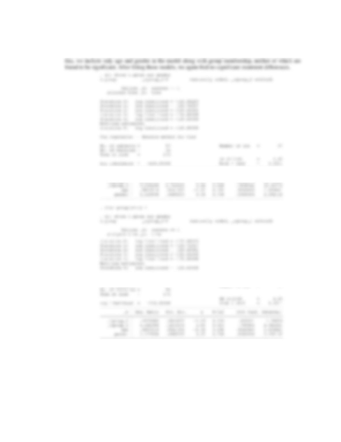
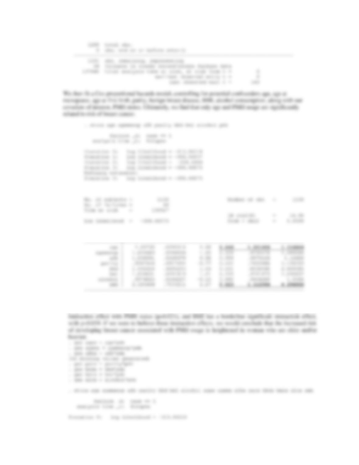
14.40 Since we are controlling for covariates, we need to use a Cox proportional hazards model. We note that,
due to the low number of events, this model cannot be fit while using “side” as a covariate. Because of
——————————————————————————
_t | Haz. Ratio Std. Err. z P>|z| [95% Conf. Interval]
————-+—————————————————————-
_Igroup_1 | 2.452794 1.844971 1.19 0.233 .5615579 10.71341
Cox regression — Breslow method for ties
No. of subjects = 57 Number of obs = 57
——————————————————————————
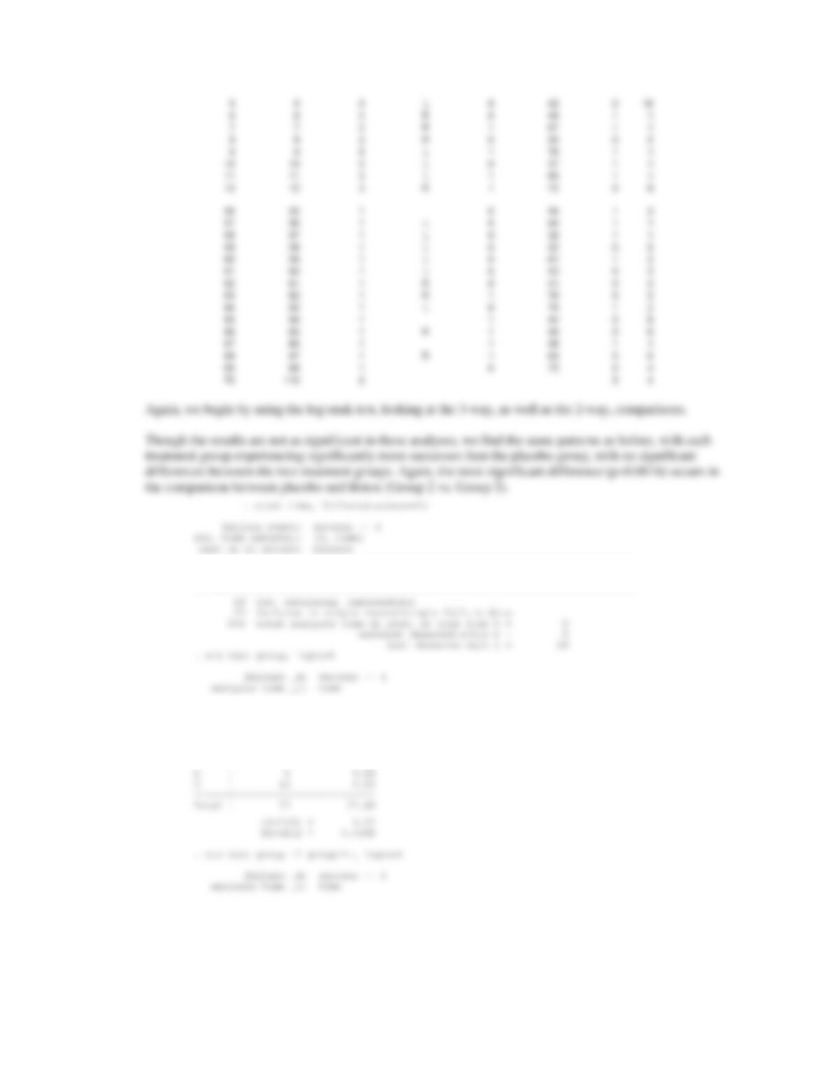
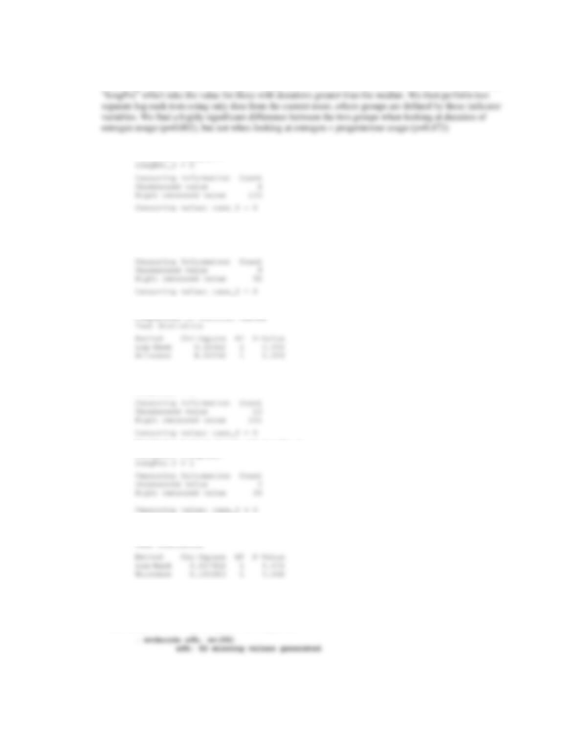
14.41 For this question, we use the new definition of success, and use for our “Time” variable, the time of the
second consecutive follow-up visit at which an improvement of at least 50% was reported. Selected
values from this new data is shown below.
Obs ID group side gender age Success Time
1 1 3 L 1 48 1 2
2 2 2 0 3
3 3 3 1 62 0 2
4 4 3 1 42 1 3
CHAPTER 14/HYPOTHESIS TESTING: PERSON-TIME DATA 435
——————————————————————————
70 total obs.
1 obs. end on or before enter()
Log-rank test for equality of survivor functions
| Events Events
group | observed expected
——+————————-
1 | 13 12.31
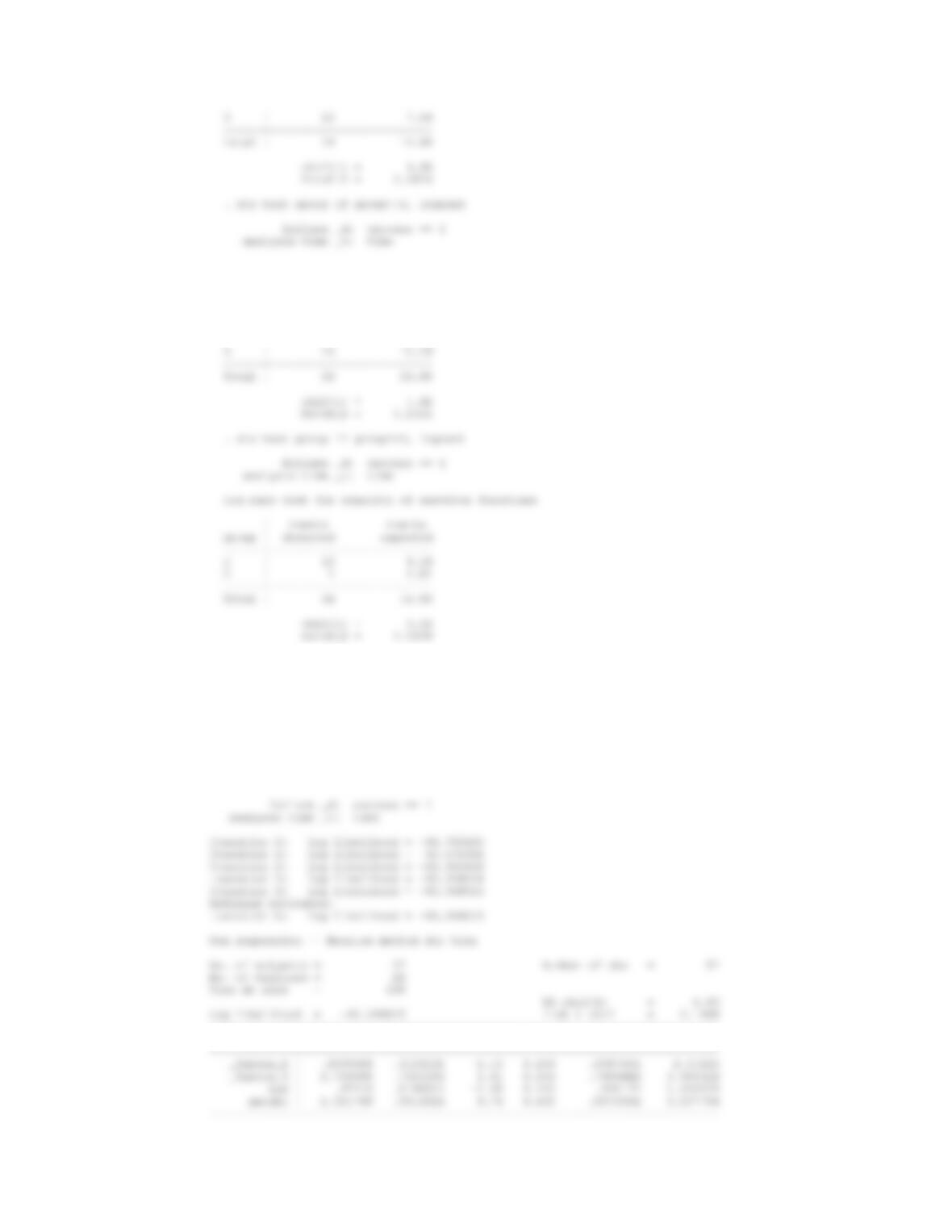
Log-rank test for equality of survivor functions
| Events Events
group | observed expected
——+————————-
2 | 1 6.46
436 CHAPTER 14/HYPOTHESIS TESTING: PERSON-TIME DAT
A
Log-rank test for equality of survivor functions
| Events Events
group | observed expected
——+————————-
1 | 13 15.71
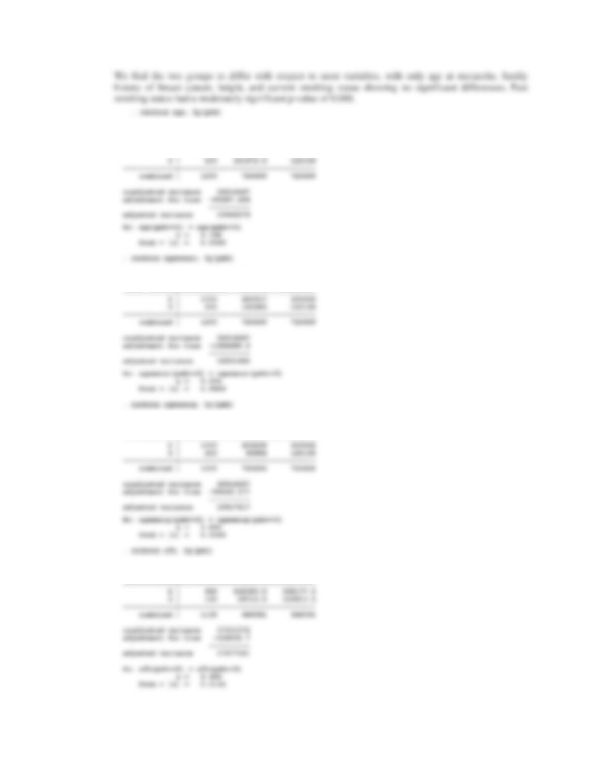
14.42 Again fitting a Cox proportional hazards regression model to our new data (using age and gender as
covariates), we find no significant treatment differences, though the comparison between the Botox
group and the placebo group (Group 3 vs. Group 2) approaches significance (p=0.09), and estimates that
Botox injections are approximately 6 (CI: 0.8- 47) times more likely to result in a “success” at any given
time, relative to a placebo injection.
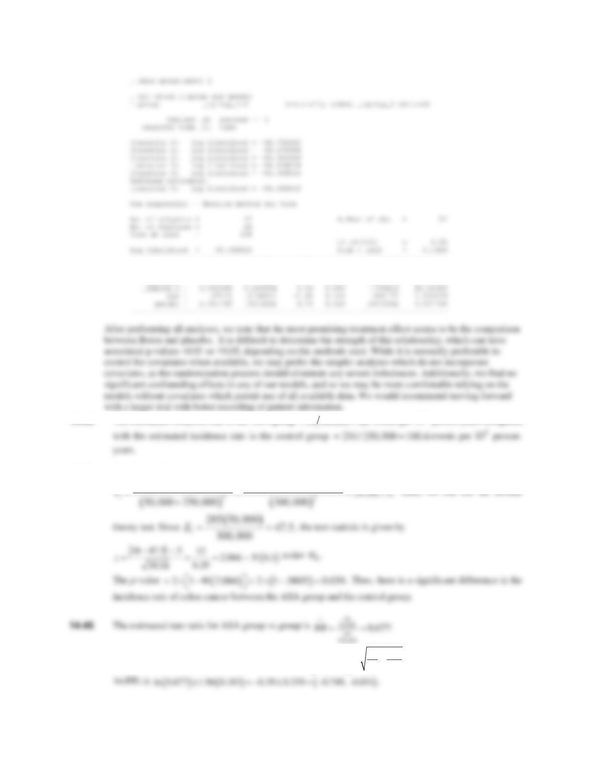
. xi: stcox i.group age gender
i.group _Igroup_1-3 (naturally coded; _Igroup_1 omitted)
——————————————————————————
_t | Haz. Ratio Std. Err. z P>|z| [95% Conf. Interval]
CHAPTER 14/HYPOTHESIS TESTING: PERSON-TIME DATA 437
——————————————————————————
_t | Haz. Ratio Std. Err. z P>|z| [95% Conf. Interval]
————-+—————————————————————-
_Igroup_1 | 3.334792 3.479857 1.15 0.248 .4313598 25.78089
14.43 The estimated incidence rate in the ASA group 34 50,000 68
events per 105 person-years compared
14.44 To compare the incidence rates we have
285 50,000 250,000 285 50,000 250,000 39.58 5.
14.46 To obtain a 95% CI for RR we first compute 11
ln 0.183
34 251
se RR
ªº
§·
¨¸
«»
©¹
¬¼
. Then, a 95% CI for
438 CHAPTER 14/HYPOTHESIS TESTING: PERSON-TIME DAT
A
14.47 In this case, we have
We have
12
2, 20,
aa
14.48 The estimated mortality rate for current smokers is 3602/420,761 = 8.56 per 1000 person-years.
14.50 To compare the mortality rates we have
(889 3602) 124,095 420,761 (4491) 124,095 420,761 789.9
14.51 The estimated rate ratio for former smokers who quit 20+ years ago vs. current smokers is
14.52 Yes, the age-adjusted rate ratio of 0.34 is lower than the crude rate ratio of 0.59 because age is a positive
CHAPTER 14/HYPOTHESIS TESTING: PERSON-TIME DATA 439
14.54 For each group, the 10-year survival probability is estimated by
1
ˆ(10) (1 )
j
j
d
SS
.
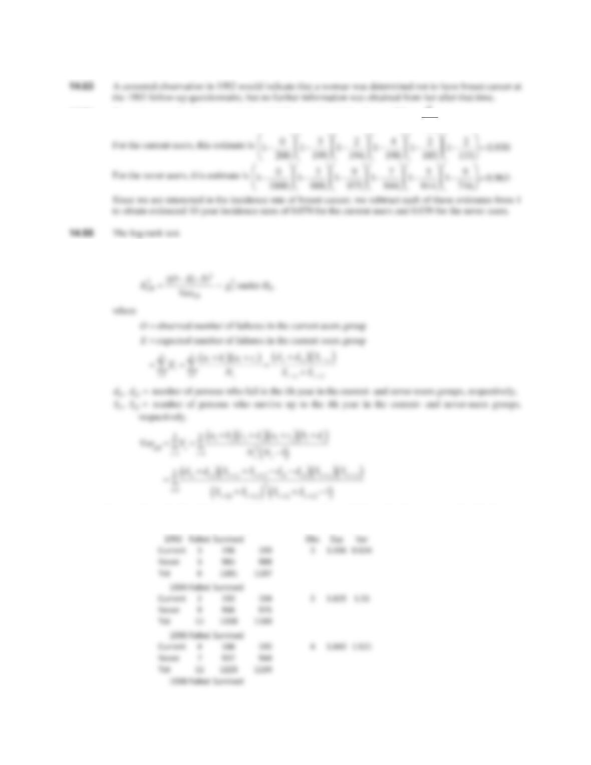
14.56 For our log-rank test, we have the test statistic
We note that at the first time point (1990), there are no observed failures in either group, and so the data
from 1990 do not contribute to the log-rank test. The remaining data is shown below.
440 CHAPTER 14/HYPOTHESIS TESTING: PERSON-TIME DAT
A
14.57 The hazard rate in this study is the instantaneous probability of death from COPD for any person who is
currently alive at a given time.
14.58 The proportional hazards model is written
h(t) h
0
(t)exp(
E
j
x
j
)
¦
, where h(t) refers to the hazard rate
for a particular person with covariates (x) at a given time t. Here, h0(t) refers to a baseline hazard
function, and coefficients Ⱦj describe the effect of each individual covariate xj on the overall hazard.
“Proportional hazards” refers to the assumption that the effect of any given covariate on the hazard
14.59 The hazard ratio is estimated to be exp(0.166) = 1.18, with a 95% confidence interval of
14.60 For this comparison, we assume the observed effect of smoking for men and women are both normally
CHAPTER 14/HYPOTHESIS TESTING: PERSON-TIME DATA 441
So then,
14.62 In order to have 90% for this type of study we would require
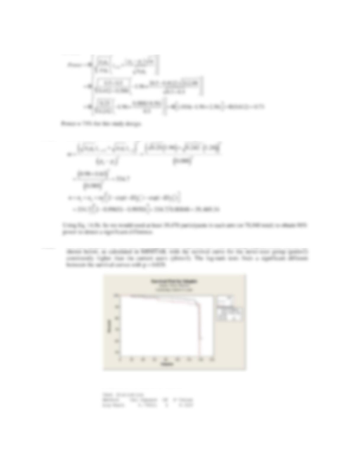
14.63 For this analysis, we will use the nonparametric log-rank test. The resulting Kaplan-Meier curves are
Distribution Analysis: foluptm by pmh
Comparison of Survival Curves
442 CHAPTER 14/HYPOTHESIS TESTING: PERSON-TIME DAT
A
14.64 For this analysis, we calculate the median duration of use among the current PMH users to be 48 months
for estrogen and 24 months for estrogen + progesterone. We then create indicator variables “longEst” and
Distribution Analysis: foluptm_3 by longEst_3
Variable: foluptm_3
Distribution Analysis: foluptm_3 by longEst_3
Variable: foluptm_3
longEst_3 = 1
Distribution Analysis: foluptm_3 by longEst_3
Distribution Analysis: foluptm_3 by longPro_3
Variable: foluptm_3
longPro_3 = 0
Distribution Analysis: foluptm_3 by longPro_3
Variable: foluptm_3
Distribution Analysis: foluptm_3 by longPro_3
Comparison of Survival Curves
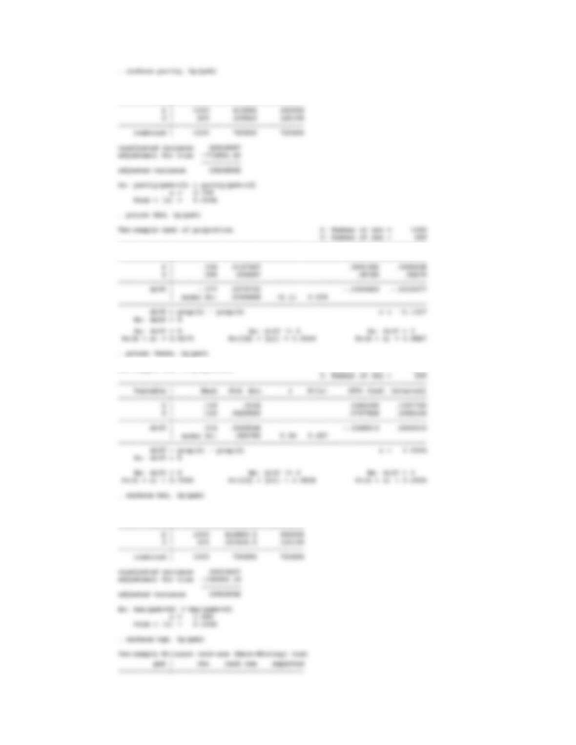
14.65 Below, we use STATA to compare the two groups with respect to all available covariates, using two-
sample binomial tests and non-parametric Wilcoxon rank-sum test for all other variables, using the .prtest
and .ranksum commands. First, we make sure to recode the values in column ‘afb’ so that values of 98
are changed to missing, using the following code.
CHAPTER 14/HYPOTHESIS TESTING: PERSON-TIME DATA 443
Two-sample Wilcoxon rank-sum (Mann-Whitney) test
pmh | obs rank sum expected
————-+———————————
2 | 1000 619123.5 600500
Two-sample Wilcoxon rank-sum (Mann-Whitney) test
pmh | obs rank sum expected
Two-sample Wilcoxon rank-sum (Mann-Whitney) test
pmh | obs rank sum expected
————-+———————————
Two-sample Wilcoxon rank-sum (Mann-Whitney) test
pmh | obs rank sum expected
444 CHAPTER 14/HYPOTHESIS TESTING: PERSON-TIME DAT
A
Two-sample Wilcoxon rank-sum (Mann-Whitney) test
pmh | obs rank sum expected
——————————————————————————
Variable | Mean Std. Err. z P>|z| [95% Conf. Interval]
Two-sample test of proportion 2: Number of obs = 1000
Two-sample Wilcoxon rank-sum (Mann-Whitney) test
pmh | obs rank sum expected
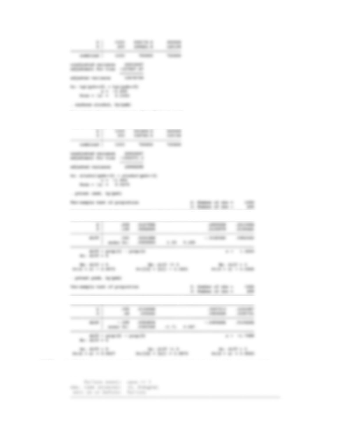
CHAPTER 14/HYPOTHESIS TESTING: PERSON-TIME DATA 445
Two-sample Wilcoxon rank-sum (Mann-Whitney) test
pmh | obs rank sum expected
————-+———————————
——————————————————————————
Variable | Mean Std. Err. z P>|z| [95% Conf. Interval]
——————————————————————————
Variable | Mean Std. Err. z P>|z| [95% Conf. Interval]
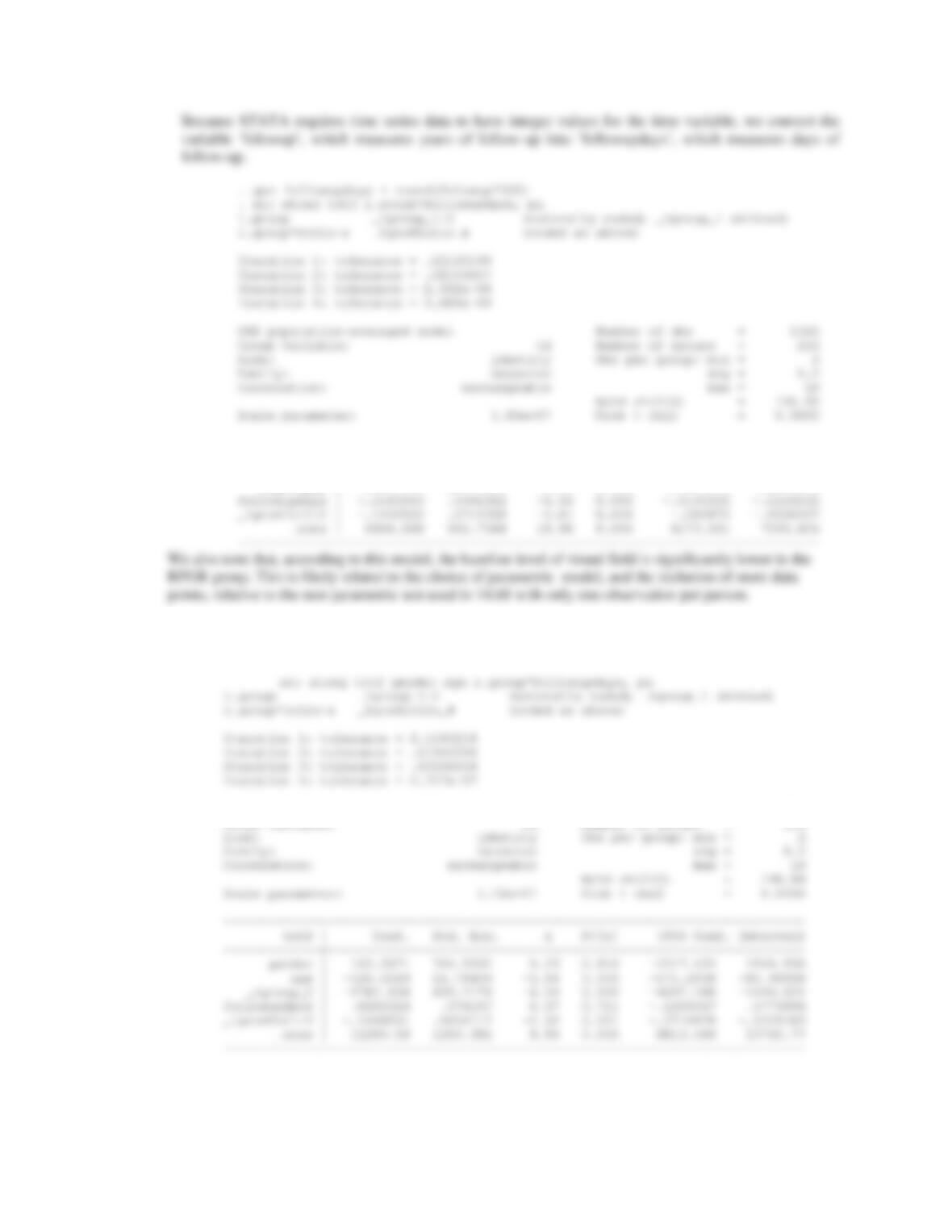
14.66 In STATA, we first have to format our data as survival data using the following command.
stset foluptm, failure(case==1)
446 CHAPTER 14/HYPOTHESIS TESTING: PERSON-TIME DAT
A
Cox regression — Breslow method for ties
——————————————————————————
_t | Haz. Ratio Std. Err. z P>|z| [95% Conf. Interval]
14.67 For this analysis, we create interaction terms for each of our potential confounders and then refit the Cox
proportional hazards model with all of our new covariates. We now find that age has a significant
CHAPTER 14/HYPOTHESIS TESTING: PERSON-TIME DATA 447
——————————————————————————
_t | Haz. Ratio Std. Err. z P>|z| [95% Conf. Interval]
————-+—————————————————————-
age | .7542263 .1129113 -1.88 0.060 .5624355 1.011418
agemenop | .8116765 .1384321 -1.22 0.221 .5810451 1.133851
——————————————————————————
14.68 To compare baseline visual field levels, we perform a Wilcoxon rank-sum test on the calculated
geometric mean visual field values Totf= sqrt(totfldod x totfldos), restricting our data to those values
with folowup=0, indicating that the data was collected at baseline. We find no significant differences
between the two groups.
group | obs rank sum expected
————-+———————————
14.69 Using GEE methods from Chapter 13, we can fit a population-average model which accounts for the
correlation in the observations within each individual. Including an interaction term between the effect of
448 CHAPTER 14/HYPOTHESIS TESTING: PERSON-TIME DAT
A
——————————————————————————
totf | Coef. Std. Err. z P>|z| [95% Conf. Interval]
————-+—————————————————————-
_Igroup_2 | -1609.433 568.4829 -2.83 0.005 -2723.639 -495.2269
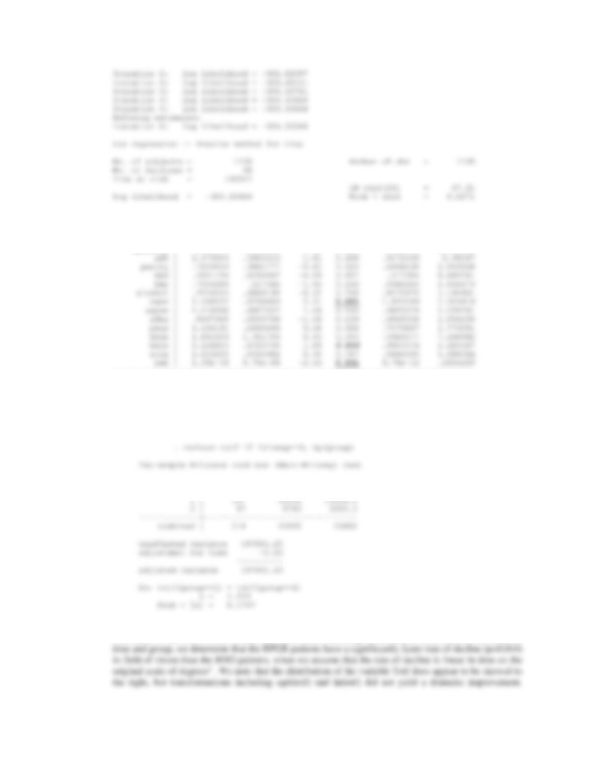
14.70 After accounting for gender and age, we now find an even more significant difference in the rates of
decline in visual field in the RPGR group, with p=0.021.
GEE population-averaged model Number of obs = 1326
Group variable: id Number of groups = 214
14.71 There is quite a bit of data manipulation that must be performed to prepare for this analysis, which we
choose to perform using the log-rank test. It is possible to reshape the data in MINITAB, creating
CHAPTER 14/HYPOTHESIS TESTING: PERSON-TIME DATA 449
indicators of group membership, indicators of blindness, maximum time under observation, etc. for each
individual, by repeatedly using the “store summary statistics” command.
. gen blind = (totf<314)
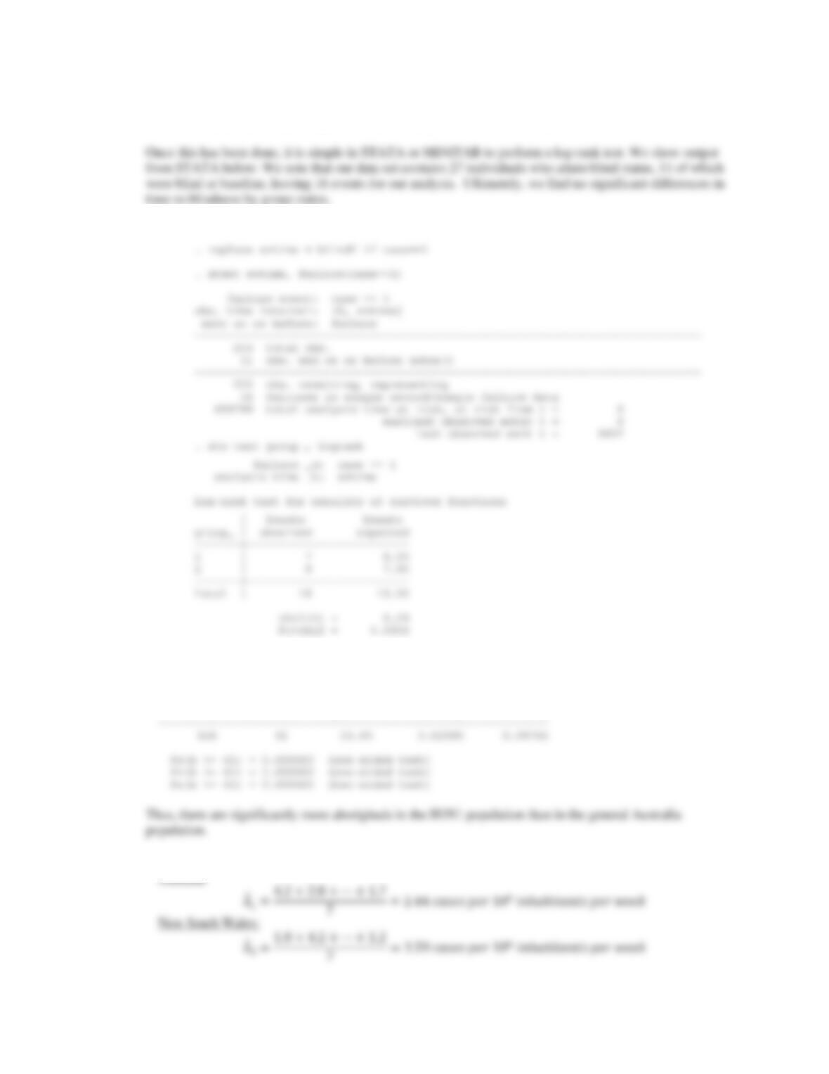
14.72 We reject the null hypothesis with a p-value < 0.0001
. bitesti 626 61 0.025
N Observed k Expected k Assumed p Observed p
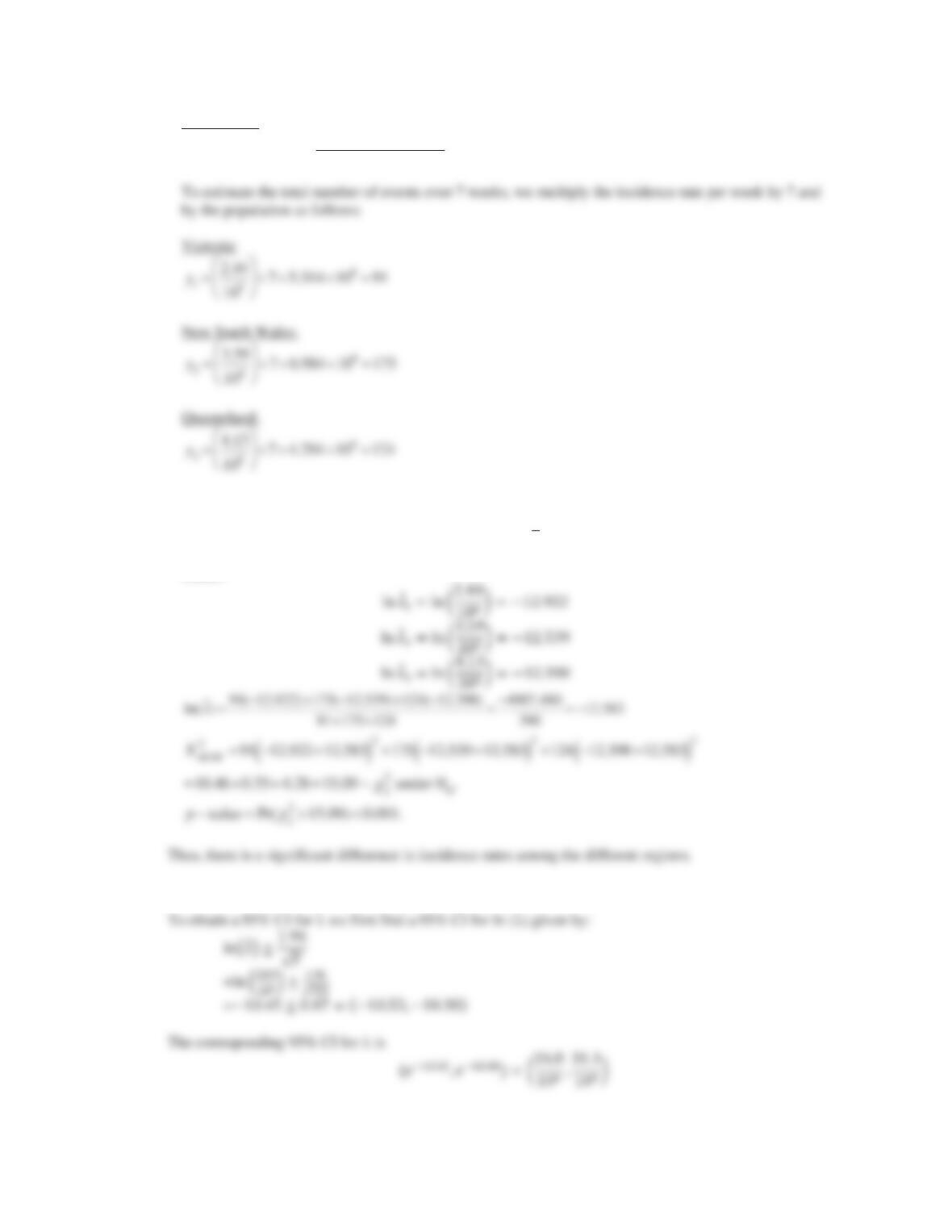
14.73 The incidence rate per million inhabitants per week by region was as follows:
Victoria: ߣመଵൌͶǤʹʹǤͺڮͳǤ
450 CHAPTER 14/HYPOTHESIS TESTING: PERSON-TIME DAT
A
Queensland: ߣመଷൌͲǤʹͲǤͺڮͷǤʹ
ൌͶǤͳ͵ܿܽݏ݁ݏ݁ݎͳͲ݄ܾ݅݊ܽ݅ݐܽ݊ݐݏ݁ݎݓ݁݁݇
14.74 To test for homogeneity across different strata, we use the test statistic:
ܺுைெ
ଶൌݕሺ݈݊ߣመ
ଷ
ୀଵ െ݈݊ߣሻଶ̱ݔଶ
ଶݑ݊݀݁ݎܪ
where: ߣመൌ൬ʹǤͶͶ
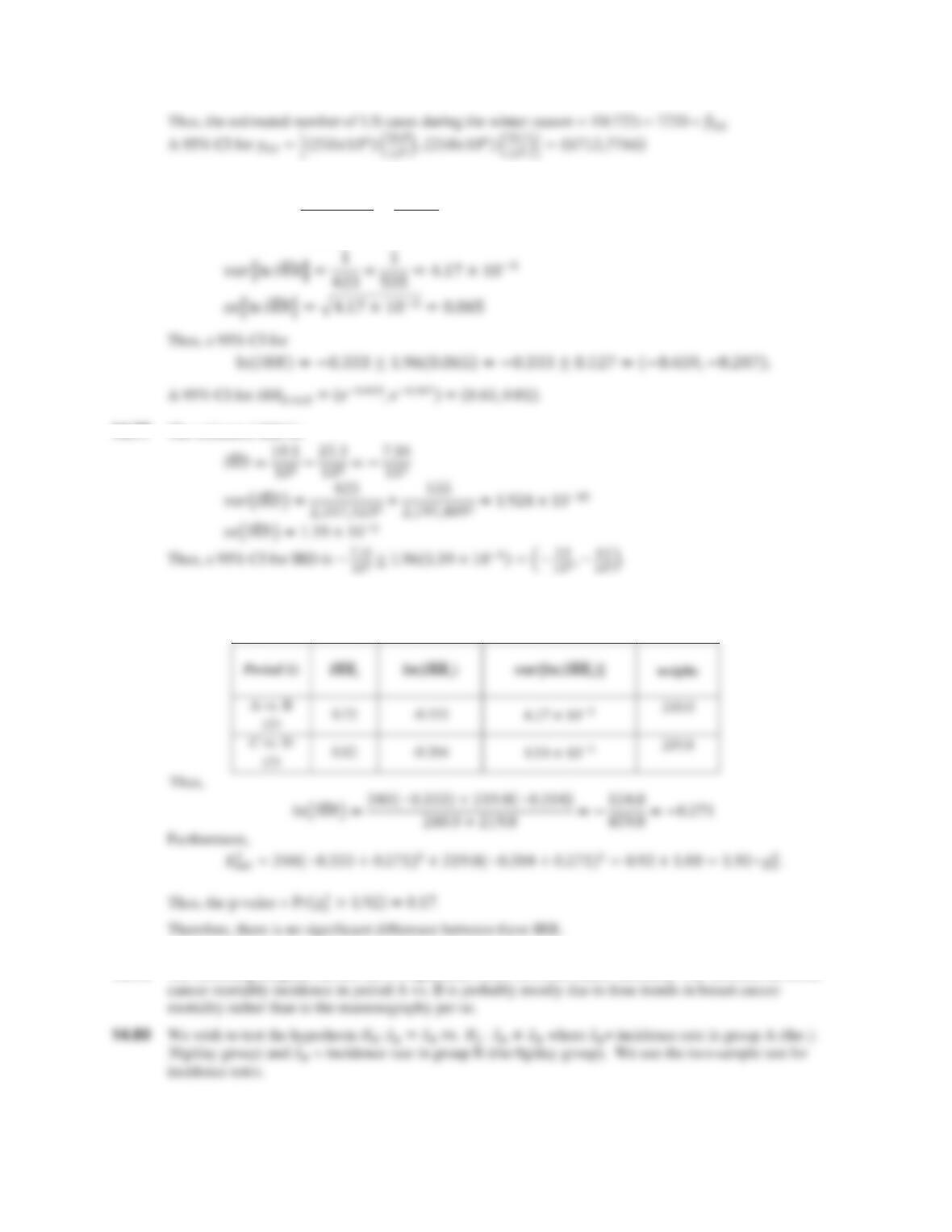
14.75 The estimated incidence rate in Australia =
722 / (25 x 10
6
) 28.9 /10
6
ˆ
O
.
CHAPTER 14/HYPOTHESIS TESTING: PERSON-TIME DATA 451
14.76
୴ୱǤ ൌସଶଷȀଶǡଷଷǡଷଶଷ
ହହହȀଶǡଵଽǡସସൌଵ଼ǤଵȀଵఱ
ଶହǤଷȀଵఱൌͲǤʹ
ܫܴܴ
ൌെͲǤ͵͵͵
14.77 The estimated IRD is:
14.78 We must assess the homogeneity of ܫܴܴ௩௦Ǥ and ܫܴܴ௩௦ǤǤ
We have the following results:
14.79 The screening program did not have a significant effect in breast cancer mortality. The decrease in breast
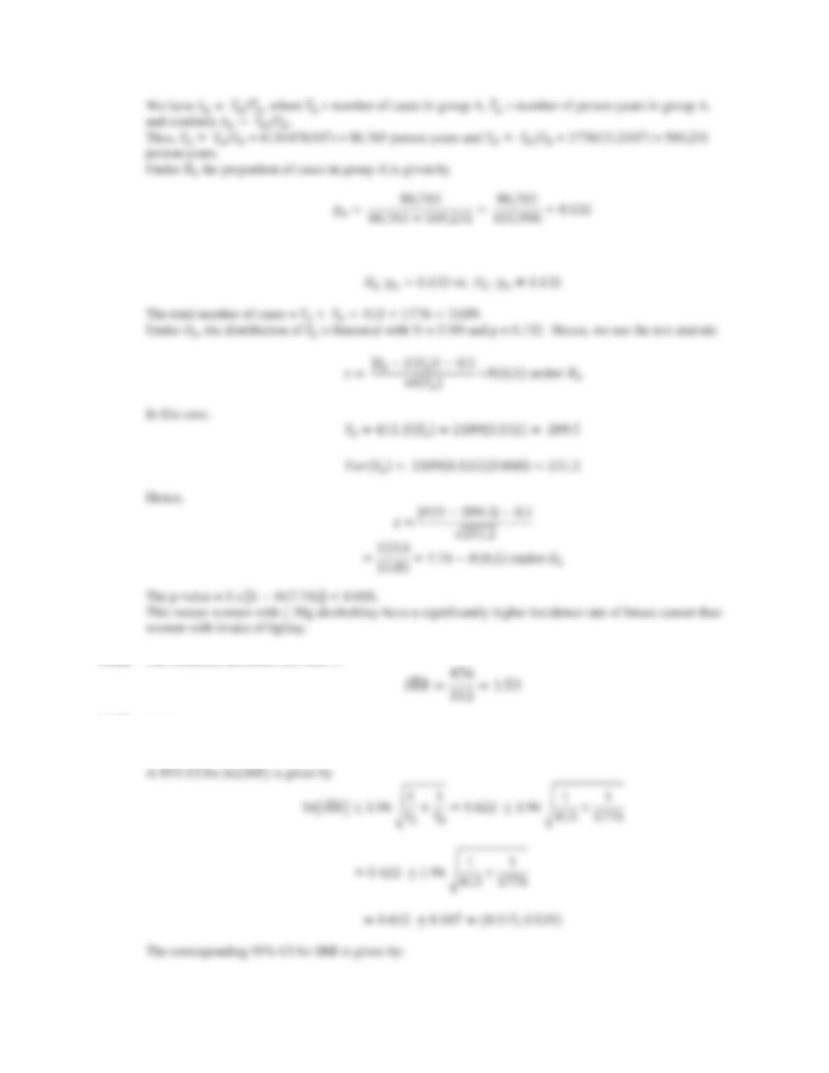
14.81 We need to compute the person-years in groups A and B, respectively.
452 CHAPTER 14/HYPOTHESIS TESTING: PERSON-TIME DAT
A
The test is equivalent to a one-sample binomial test, where
ܪǣൌͲǤͳ͵ʹǤܪଵǣ്ͲǤͳ͵ʹ
14.82 The estimated incidence rate ratio is ܫܴܴ
14.83 We have:
݈݊ሺܫܴܴ
ሻൌͲǤͶʹʹ
CHAPTER 14/HYPOTHESIS TESTING: PERSON-TIME DATA 453
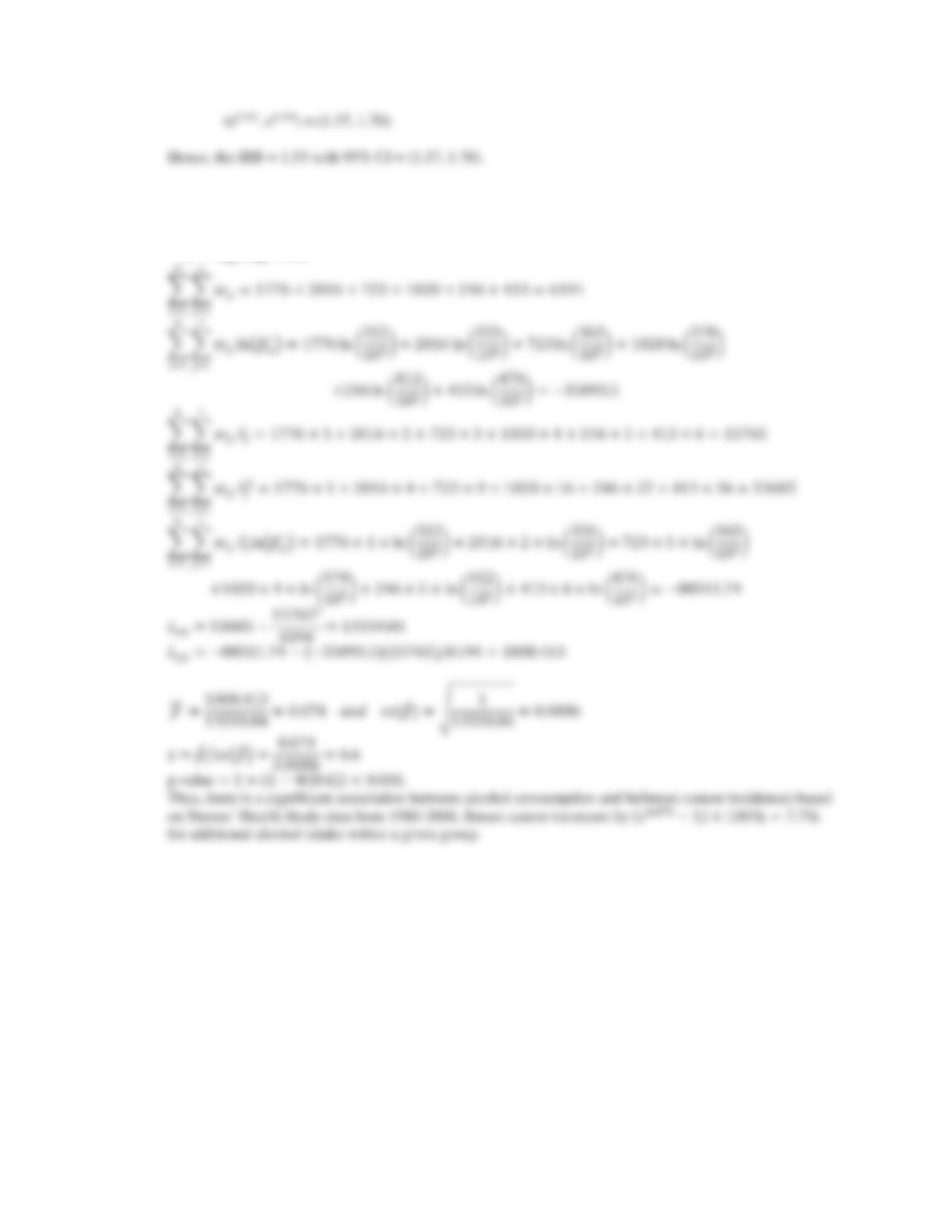
14.84 We consider, as in Equation 14.27 (in Chapter 14, text), a model of the form
൫൯ൌߙߚܵ
We want to test the hypothesis ܪǣߚൌͲ versus ܪଵǣߚ്Ͳ. The point estimate of ߚ is given by
ߚመൌܮ௫௬ ܮ௫௫
Τ where