414
HYPOTHESIS TESTING:
PERSON-TIME
DATA
14.1 The incidence density among current users 13 4761 2731. cases per 105 person-years. The incidence
14.2 The incidence density among past users 164 121 091 135 4,. cases per 105 person-years compared
14.3 The estimated rate ratio for current users vs never users is RR
13
4761
113
98 091
237
,
.. To obtain a 95% CI for RR
CHAPTER 14/HYPOTHESIS TESTING: PERSON-TIME DATA 415
14.4 The estimated rate ratio for past users vs never users is RR
164
121 091
113
118
,
.. To obtain a 95% CI for RR,
14.5 We refer to Equation 14.12 (in Chapter 14, text). We have:
D
.05
Thus,
14.6 We can solve for m from Equation 14.12 as follows:
416 CHAPTER 14/HYPOTHESIS TESTING: PERSON-TIME DAT
A
Solving for m we obtain:
14.7 For this data, we create the indicator variable ‘Above’, which takes the value 1 if adjusted log(CO) >
14.8 Output from MINITAB is shown below, including summary statistics for each group, and results from
CHAPTER 14/HYPOTHESIS TESTING: PERSON-TIME DATA 417
IQR = 126 Q1 = 3 Q3 = 129
Distribution Analysis: Day_abs by Above
Variable: Day_abs
Above = 1
IQR = 39 Q1 = 2 Q3 = 41
14.9 We compute
z
i
ˆ
E
i
se ˆ
E
i
and the corresponding p-value is
p 2u1) z
i
ª
¼
¼
for each of the risk factors
as follows
Risk Factor Test Statistic p-value
Age 0.40 NS
14.10 We compute the estimated hazard ratio for recidivism after taking other factors into account comparing
Risk factor
‘
Odds ratio 95% CI
Age 10 1.02 (0.91, 1.15)
14.11 After controlling for additional covariates in 14.9 and 14.10, we find a stronger relationship between CO
418 CHAPTER 14/HYPOTHESIS TESTING: PERSON-TIME DAT
A
14.12 We use the following data set, where ‘Ratio_’ variables are calculated as ‘Wk_’ level / average(baseline
levels). Bio50 and Bio100 refer to the first time point at which ‘Ratio_’ > 1.5 or 2.0, and Bio50C and
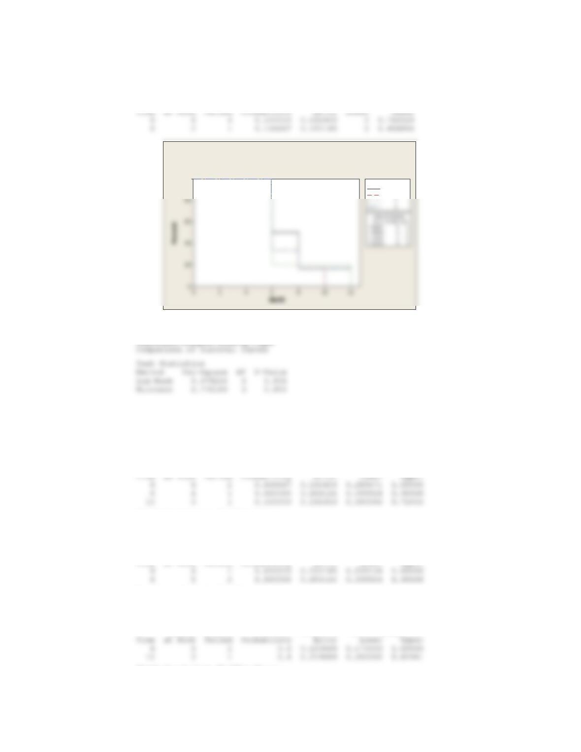
Bio100C are censoring variables for those who never meet the criteria of bioavailability. Kaplan-Meier
estimated probabilities and survival curve are shown below.
Ratio6 Ratio8 Ratio10 Ratio12 Prepar Bio50 Bio100 Bio50C Bio100C
0.84058 0.859903 1.05314 0.917874 1 12 12 1 1
2.177778 2.059259 1.807407 1.940741 1 6 6 0 0
Distribution Analysis: Bio50 by Prepar
Variable: Bio50
Prepar = 1
Number Number Survival Standard 95.0% Normal CI
Distribution Analysis: Bio50 by Prepar
Variable: Bio50
Prepar = 2
Number Number Survival Standard 95.0% Normal CI
Time at Risk Failed Probability Error Lower Upper
Distribution Analysis: Bio50 by Prepar
Variable: Bio50
Prepar = 3
Number Number Survival Standard 95.0% Normal CI
Time at Risk Failed Probability Error Lower Upper
CHAPTER 14/HYPOTHESIS TESTING: PERSON-TIME DATA 419
Distribution Analysis: Bio50 by Prepar
Variable: Bio50
Prepar = 4
Number Number Survival Standard 95.0% Normal CI
100
1
2
Prepar
Survival Plot for Bio50
Censoring Column in Bio50C
Kaplan-Meier Method
14.13 Using the log-rank test, we have no evidence of differences between preparations.
Distribution Analysis: Bio50 by Prepar
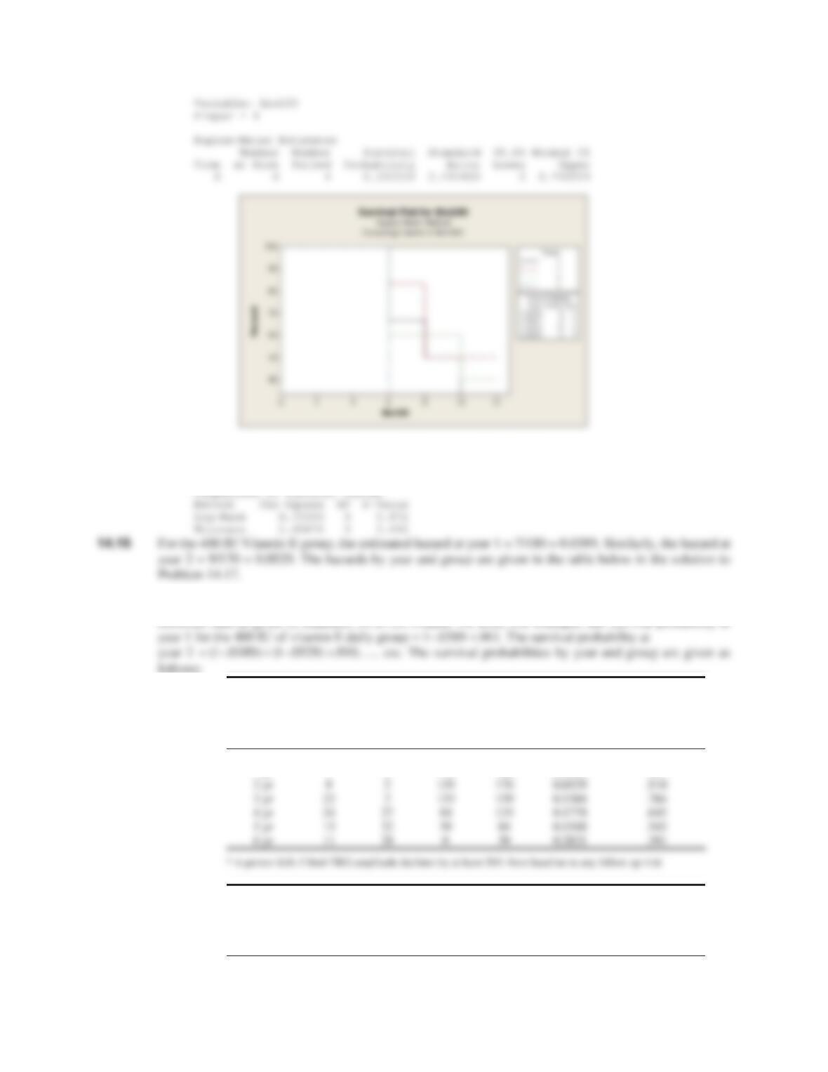
14.14 Below, we show the same output as in 14.12, using Bio100 rather than Bio50 as the variable of
interest.
Distribution Analysis: Bio100 by Prepar
Variable: Bio100
Prepar = 1
Number Number Survival Standard 95.0% Normal CI
Distribution Analysis: Bio100 by Prepar
Variable: Bio100
Prepar = 2
Kaplan-Meier Estimates
Number Number Survival Standard 95.0% Normal CI
Time at Risk Failed Probability Error Lower Upper
Distribution Analysis: Bio100 by Prepar
Variable: Bio100
Prepar = 3
Kaplan-Meier Estimates
Number Number Survival Standard 95.0% Normal CI
Distribution Analysis: Bio100 by Prepar
420 CHAPTER 14/HYPOTHESIS TESTING: PERSON-TIME DAT
A
14.15 Using this definition of bioavailability, we still find no significant differences between preparations.
Distribution Analysis: Bio100 by Prepar
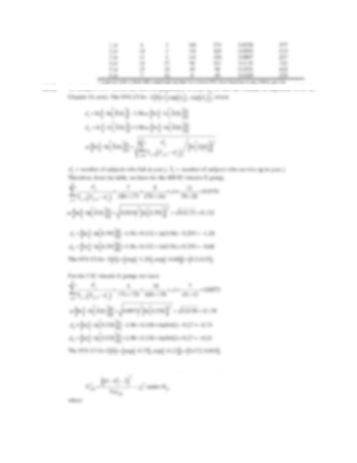
14.17 The survival probability is estimated using the Kaplan-Meier product limit estimator in the presence of
censored data as given in Equation 14.30 (in Chapter 14, text). For example, the survival probability at
follows:
Number of patients who failed, were censored or survived by year in
400 IU of vitamin E group, RP clinical trial*
Fail Censored Survive Total
Hazard at
time t
Survival
probability at
time t
400 IU of vitamin E daily
1 yr 7 3 170 180 0.0389 .961
Number of patients who failed, were censored or survived by year in
3 IU of vitamin E group, RP clinical trial*
Fail Censored Survive Total
Hazard at
time t
Survival
probability at
time t
3 IU vitamin E daily
CHAPTER 14/HYPOTHESIS TESTING: PERSON-TIME DATA 421
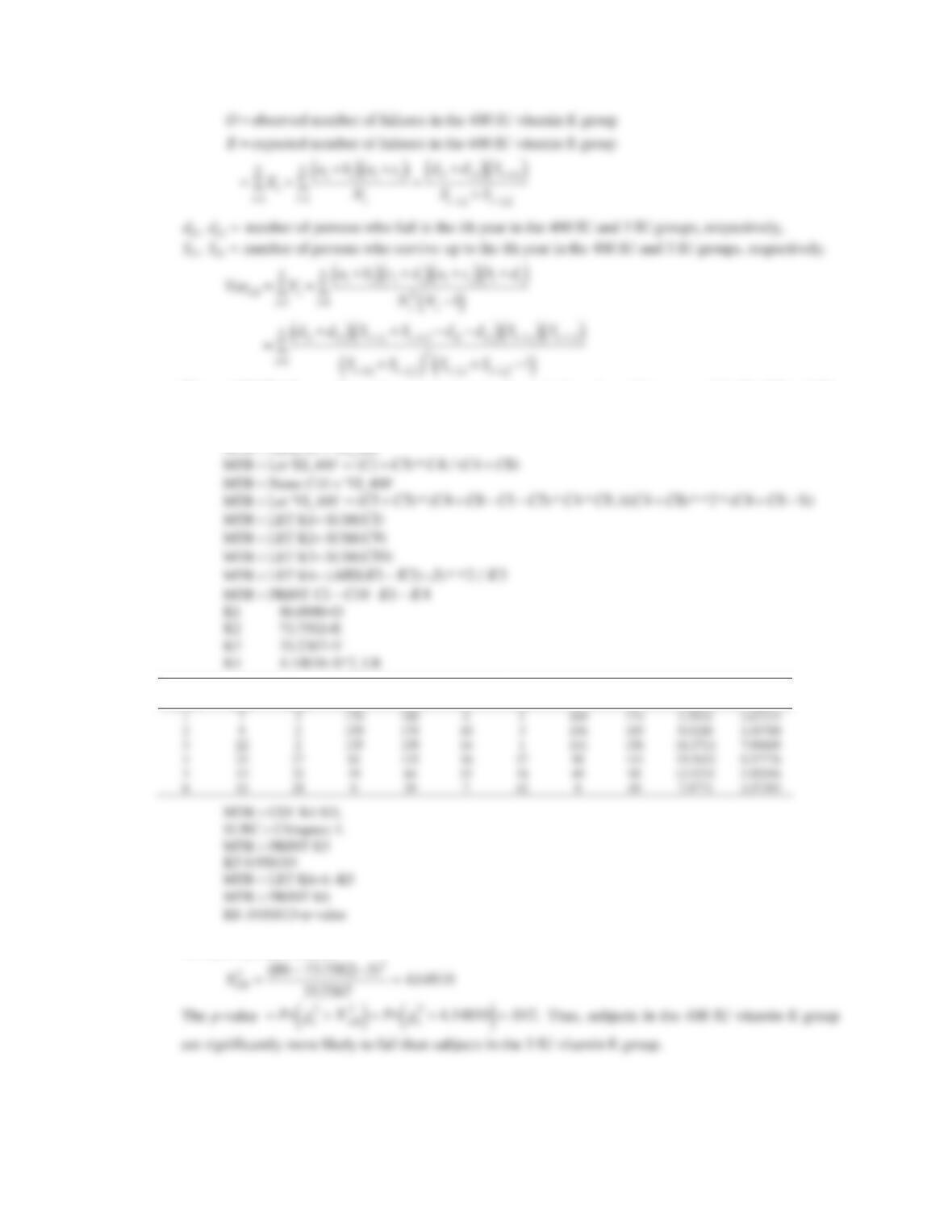
14.19 We use the log rank test procedure given in Equation 14.34 (Chapter 14, text). We have the test statistic
422 CHAPTER 14/HYPOTHESIS TESTING: PERSON-TIME DAT
A
We use MINITAB to perform the computations as shown below. EV
ii
and are stored in EIB400 and VIB
400, respectively.
ROW
FAILB
400
CENSB
400
SURVB
400
TOTB
400
FAILB
3
CENSB
3
SURVB
3
TOTB
3
EIB
400
VIB
400
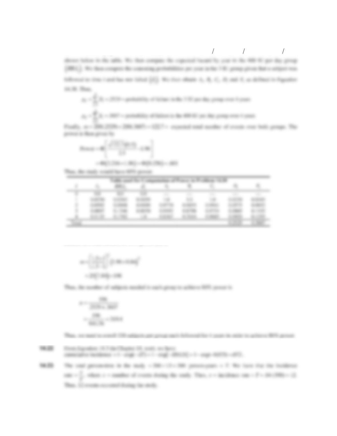
We have the test statistic
CHAPTER 14/HYPOTHESIS TESTING: PERSON-TIME DATA 423
14.20 We refer to Equation 14.38 (in Chapter 14, text) to compute the power. We first compute the hazard
function by year
O
i
in the 3 IU per day group. We have:
O
14 174 ,
O
O
24
10 169 16 141 ,, !as
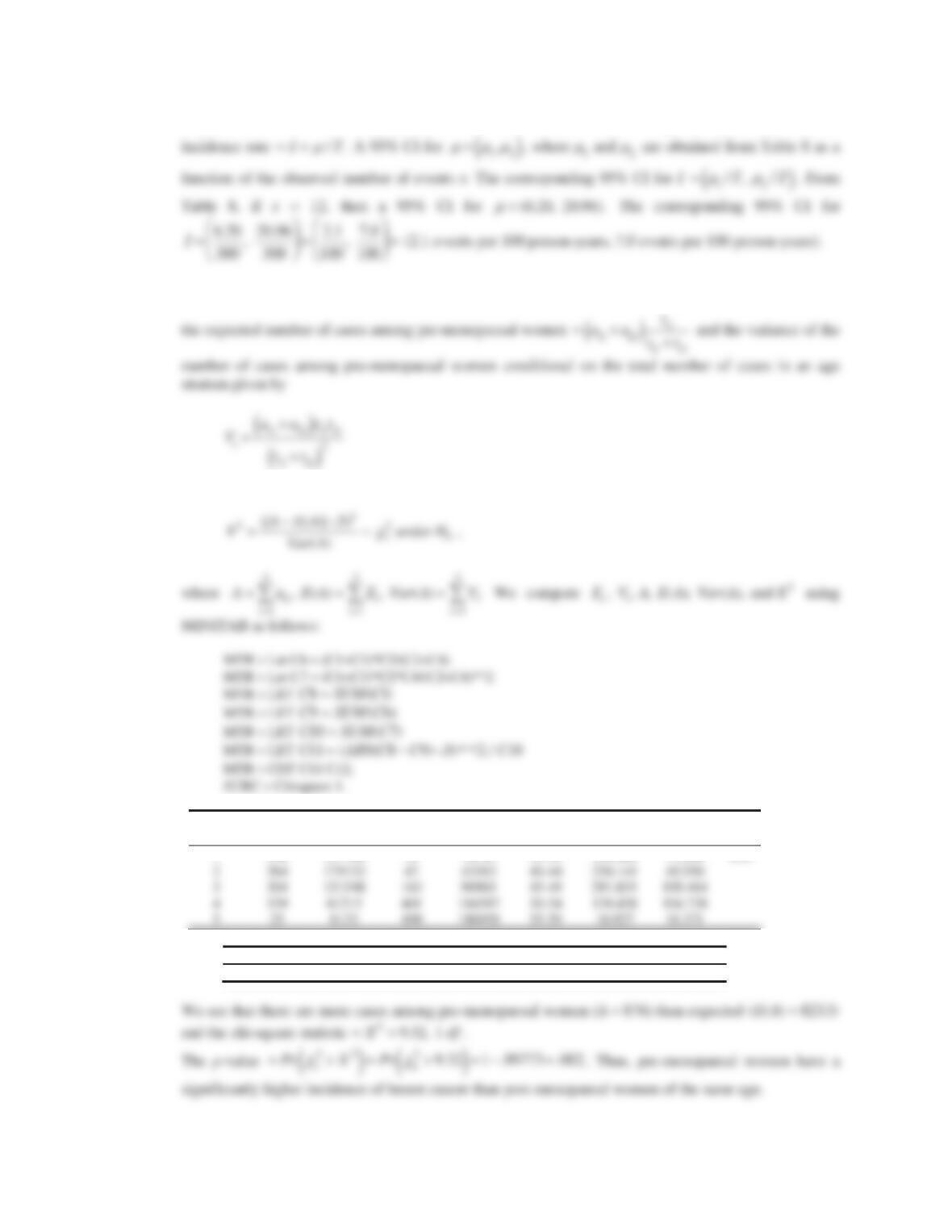
14.21 To estimate sample size we use Equation 14.39 (in Chapter 14, text). We have that the total expected
number of events needed for 80% power (m) is
O
O
G
424 CHAPTER 14/HYPOTHESIS TESTING: PERSON-TIME DAT
A
14.24 We will assume that the number of events X is Poisson distributed with expected value
P
. The true
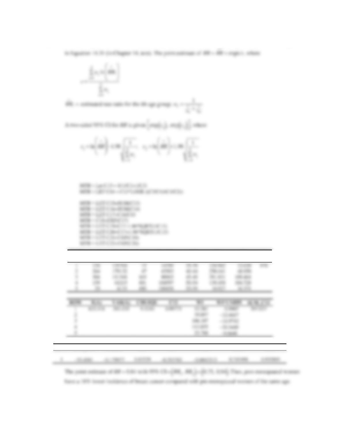
14.25 We use the test procedure in Equation 14.17 (in Chapter 14, text). For each age group, we compute Ei
We then compute the test statistic
ROW CASE
BPRE
PY-PRE CASE
BPOS
PY
B
POS AGE EI VI A
1 124 131704 15 14795 35-39 124.962 12.620 876
ROW E(A) VAR(A) CHI-SQU C12
1 823.319 292.133 9.320 0.99773
CHAPTER 14/HYPOTHESIS TESTING: PERSON-TIME DATA 425
14.26 To obtain a point and interval estimate of the rate ratio after controlling for age, we use the method given
The results obtained using MINITAB are as follows:
ROW CASE
B
PRE
PY
B
PRE CASE
B
POS
PY
B
POS AGE EI VI A
B
ROW SUM
B
C14 LN(RR)RR C1 C2 RR1RR2
426 CHAPTER 14/HYPOTHESIS TESTING: PERSON-TIME DAT
A
14.27-14.28 There are multiple methods of manipulating the data, but ultimately, we need a variable indicating
the first at which each individual became toxic, the time of the last visit for each patient, and an indicator
stset time, failure(case==1)
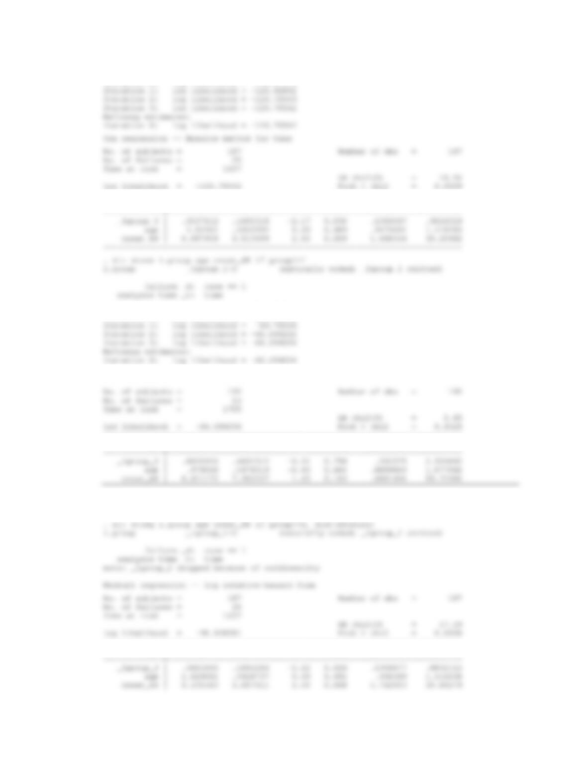
14.29-14.30 First we fit nonparametric Cox models, and again find significant differences between the high-
NAPAP group and the control group (p=0.03), and no significant difference between the low-NAPAP
CHAPTER 14/HYPOTHESIS TESTING: PERSON-TIME DATA 427
note: _Igroup_2 dropped because of collinearity
Iteration 0: log likelihood = -128.97575
——————————————————————————
_t | Haz. Ratio Std. Err. z P>|z| [95% Conf. Interval]
note: _Igroup_2 dropped because of collinearity
Iteration 0: log likelihood = -68.008061
Cox regression — Breslow method for ties
——————————————————————————
_t | Haz. Ratio Std. Err. z P>|z| [95% Conf. Interval]
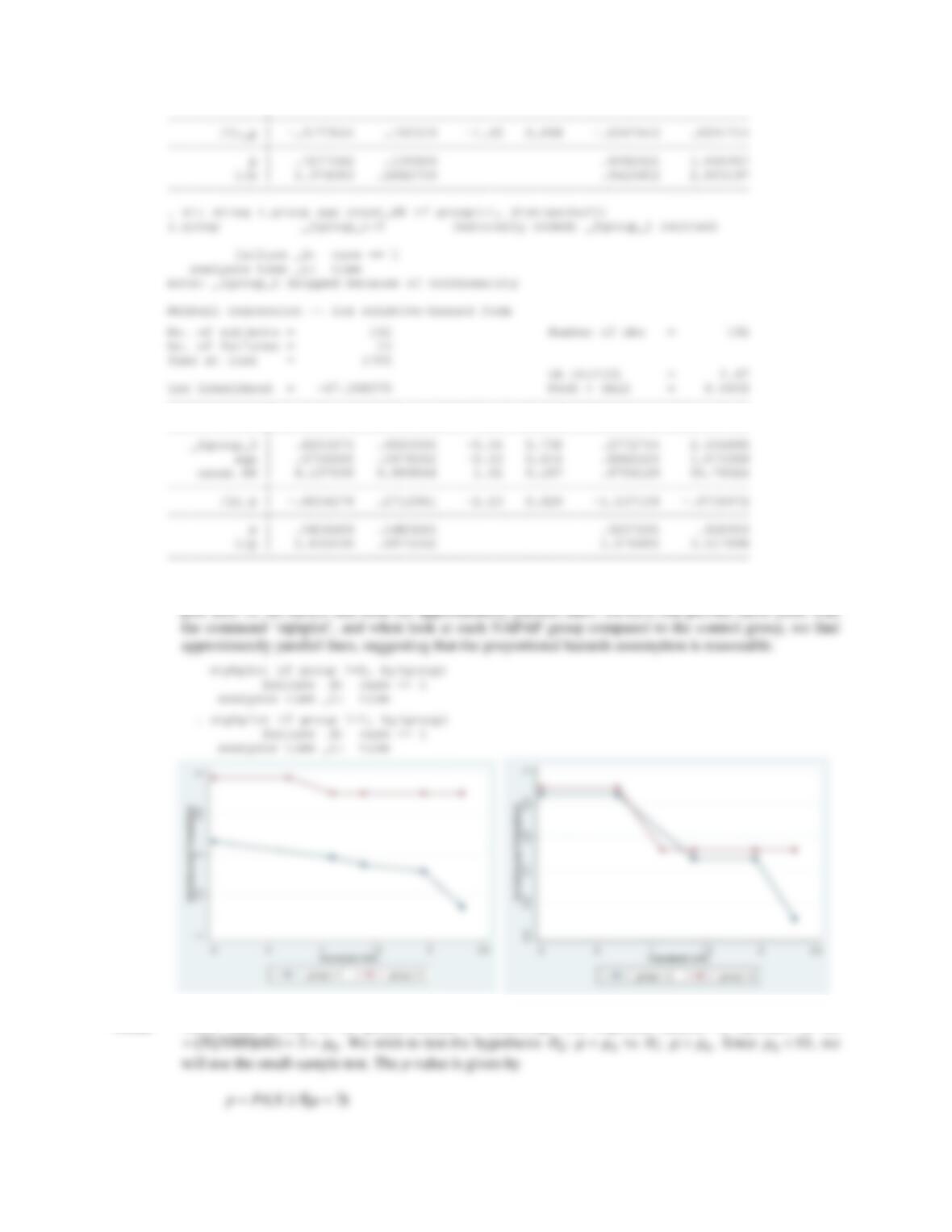
Next we fit parametric survival models using the Weibull distribution. We find the same qualitative results
as in the nonparametric models.
——————————————————————————
_t | Haz. Ratio Std. Err. z P>|z| [95% Conf. Interval]
428 CHAPTER 14/HYPOTHESIS TESTING: PERSON-TIME DAT
A
——————————————————————————
_t | Haz. Ratio Std. Err. z P>|z| [95% Conf. Interval]
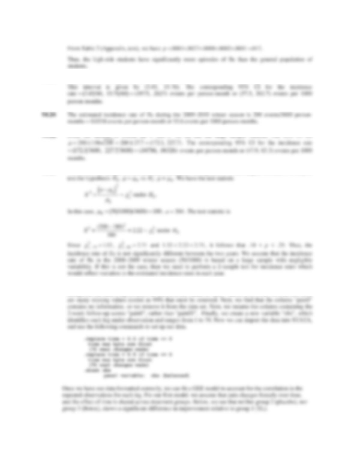
14.31 As discussed in Section 14.14, one way to assess validity of the proportional hazards assumption is to
14.32 There were a total of 60 person-months of follow-up. The expected number of episodes of flu
CHAPTER 14/HYPOTHESIS TESTING: PERSON-TIME DATA 429
14.33 Based on Table 8 (Appendix, text), we can construct a 2-sided 95% CI for
P
using x = 8 and 1.95
D
.
14.36 We use the one-sample test for incidence rates based on Equation 14.4 (in Chapter 14, text). We wish to
P
P
P
P
14.37 There are many methods which may be used to analyze this data. Before getting started, we need to
manipulate the data using STATA, so that all of the values of “pain” can be used. First, we note that there
430 CHAPTER 14/HYPOTHESIS TESTING: PERSON-TIME DAT
A
GEE population-averaged model Number of obs = 407
——————————————————————————
pain | Coef. Std. Err. z P>|z| [95% Conf. Interval]
————-+—————————————————————-
——————————————————————————
pain | Coef. Std. Err. z P>|z| [95% Conf. Interval]
————-+—————————————————————-
time | .8212945 .3544985 2.32 0.021 .1264902 1.516099
Other options for assessing the treatment effects include fitting a GEE model with time, group, and the
CHAPTER 14/HYPOTHESIS TESTING: PERSON-TIME DATA 431
Wald chi2(19) = 66.80
Scale parameter: 1189.145 Prob > chi2 = 0.0000
——————————————————————————
pain | Coef. Std. Err. z P>|z| [95% Conf. Interval]
————-+—————————————————————-
_Itime_2 | 4.052958 2.797483 1.45 0.147 -1.430007 9.535923
14.38 It is difficult to assess the impact of adding covariates to the model. We note that neither age nor gender
appears to have a significant impact on pain improvement, yet “side” is significant, with p=0.045,
. xi: xtgee pain time i.group i.side age gender
i.group _Igroup_1-3 (naturally coded; _Igroup_1 omitted)
——————————————————————————
pain | Coef. Std. Err. z P>|z| [95% Conf. Interval]
————-+—————————————————————-
time | 1.647122 .2285879 7.21 0.000 1.199097 2.095146
_Igroup_2 | -23.25588 27.79243 -0.84 0.403 -77.72803 31.21628
432 CHAPTER 14/HYPOTHESIS TESTING: PERSON-TIME DAT
A
——————————————————————————
pain | Coef. Std. Err. z P>|z| [95% Conf. Interval]
————-+—————————————————————-
time | 1.647122 .2285879 7.21 0.000 1.199097 2.095146
_Igroup_1 | 23.25588 27.79243 0.84 0.403 -31.21628 77.72803
——————————————————————————
14.39 For this question, we will use survival-analysis methods, with the outcome of interest defined as
Obs ID group side gender age Success Time
1 1 3 L 1 48 1 1
2 2 2 0 3
3 3 3 1 62 1 2
——————————————————————————
70 total obs.
1 obs. end on or before enter()
CHAPTER 14/HYPOTHESIS TESTING: PERSON-TIME DATA 433
| Events Events
group | observed expected
——+————————-
We can alternatively perform a log-rank test comparing each pair of groups with one another. Similar to
. sts test group if group!=1, logrank
Log-rank test for equality of survivor functions
| Events Events
group | observed expected
——+————————-
2 | 2 8.23
| Events Events
group | observed expected
Log-rank test for equality of survivor functions
| Events Events
group | observed expected