Ch. 14: The Production Cycle
Note: this solution was created assuming that the current year is 2011. Therefore, when using the problem in subsequent years, you may
want to have students increment all years initially placed in service by one.
Production Cycle
Useful formulas:
• Current year: =YEAR(TODAY()) – this calculates the current year. In cell E2, it is currently set to increment by 1 because
the solution was created in 2010, but designed to mimic 2011. Therefore, when using this problem in 2011 and subsequent years,
students should not increment it by 1, but simply have the formula =YEAR(TODAY()) to return the value of the current year.
• Excel has a built-in function for computing straight-line depreciation: SLN. The SLN function takes three arguments: cost,
salvage value, and estimated life: SLN(cell with cost, cell with salvage value, cell with estimated life).
Ch. 14: The Production Cycle
14.8 EXCEL PROBLEM
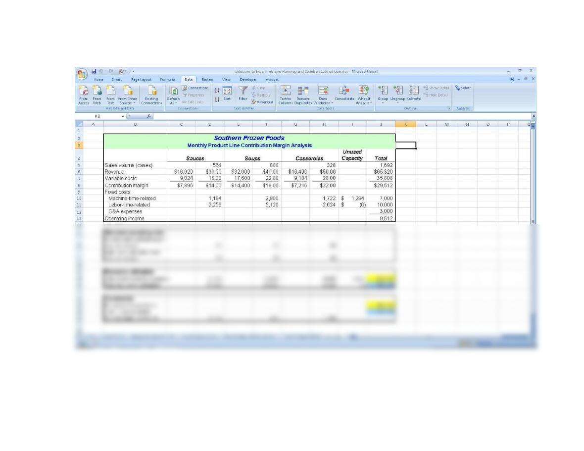
Task: Use Excel and the Solver add-in to explore the effect of various resource constraints on the optimal product mix.
a. Read the article “Boost Profits With Excel,” by James A. Weisel in the December 2003 issue of the Journal of
Accountancy (available online at the AICPA’s Web site, www.aicpa.org
b. Download the sample spreadsheet discussed in the article and print out the screenshots showing that you used the
Solver tool as discussed in the article.
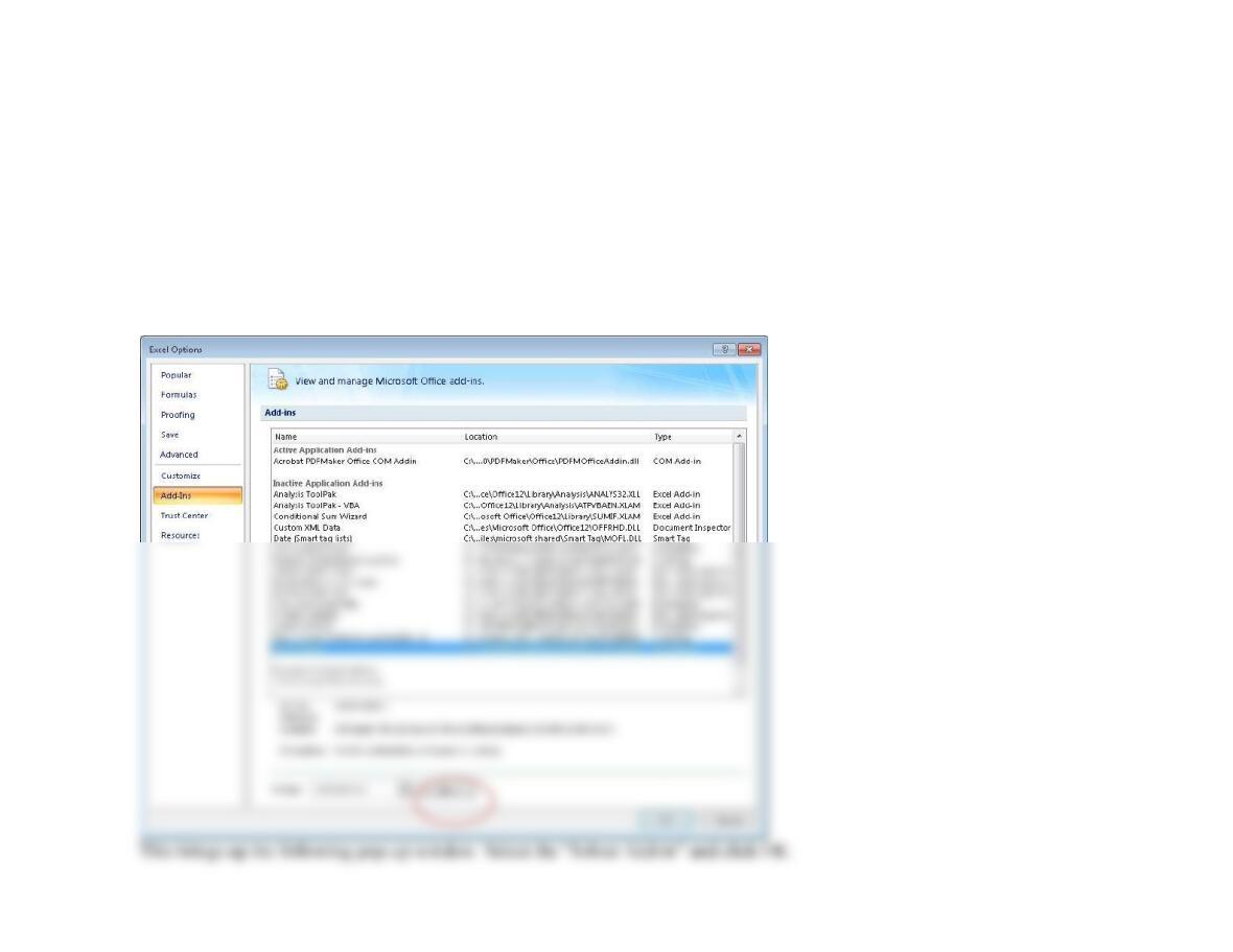
To load Solver in Excel 2007, click on the “Microsoft Office Button” in the upper left corner of an Excel spreadsheet. Then click on
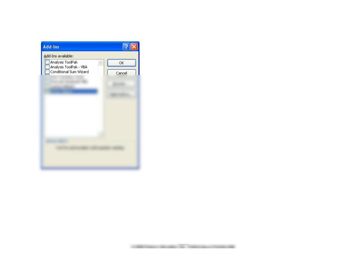
Excel Options to open the following screen, select Add-Ins, highlight “Solver Add–in” and click the “Go” button:
Production Cycle
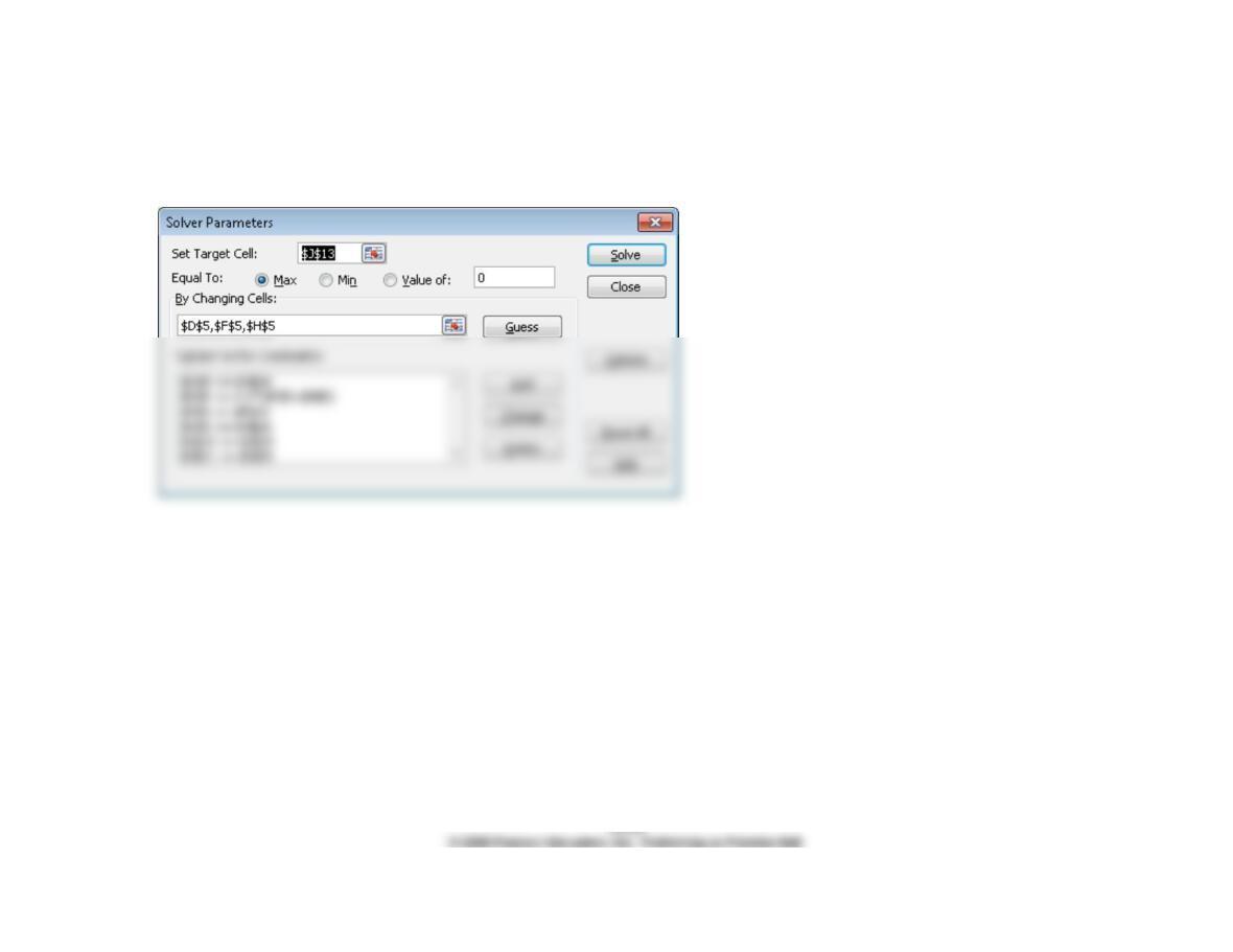
Then, to use Solver:
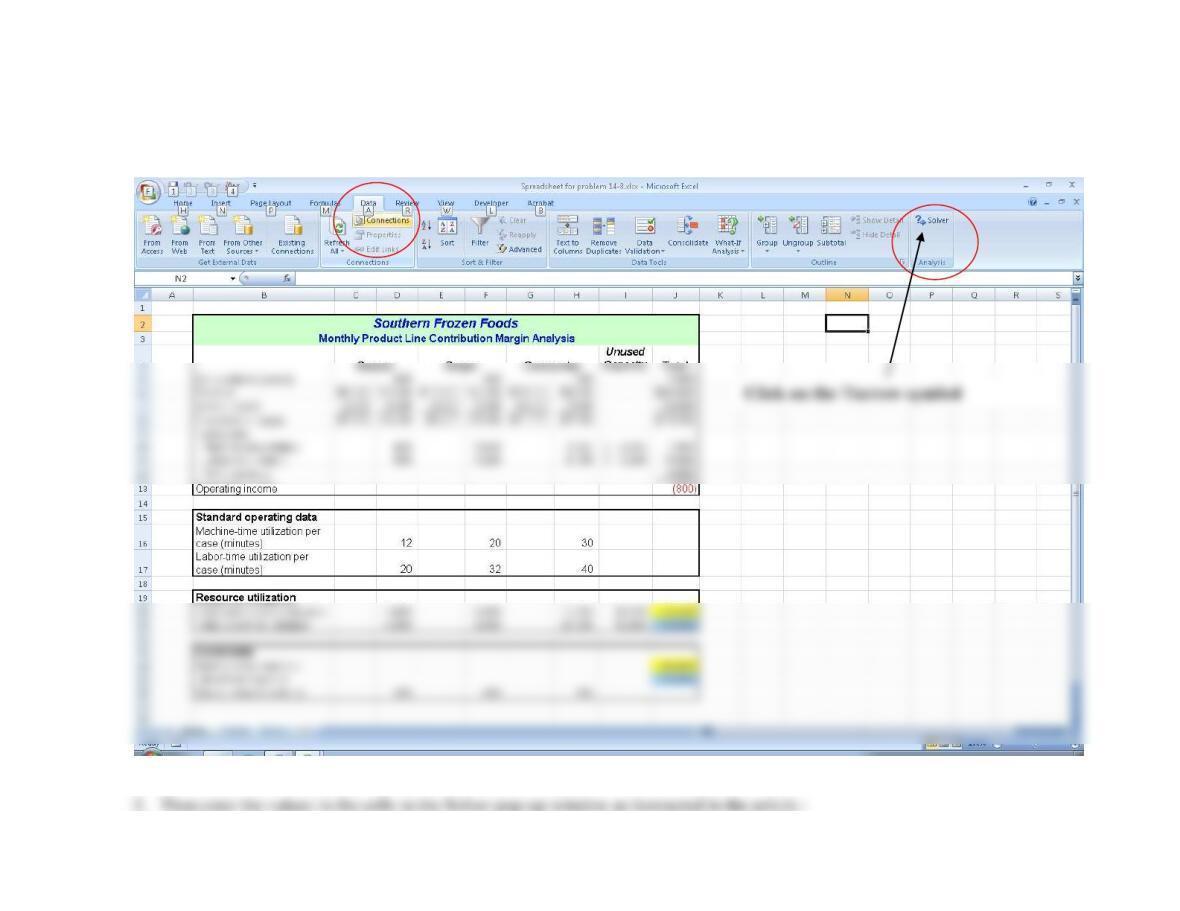
Ch. 14: The Production Cycle
1. Move to the Data tab and then click on ?/arrow symbol in the Solver
Production Cycle
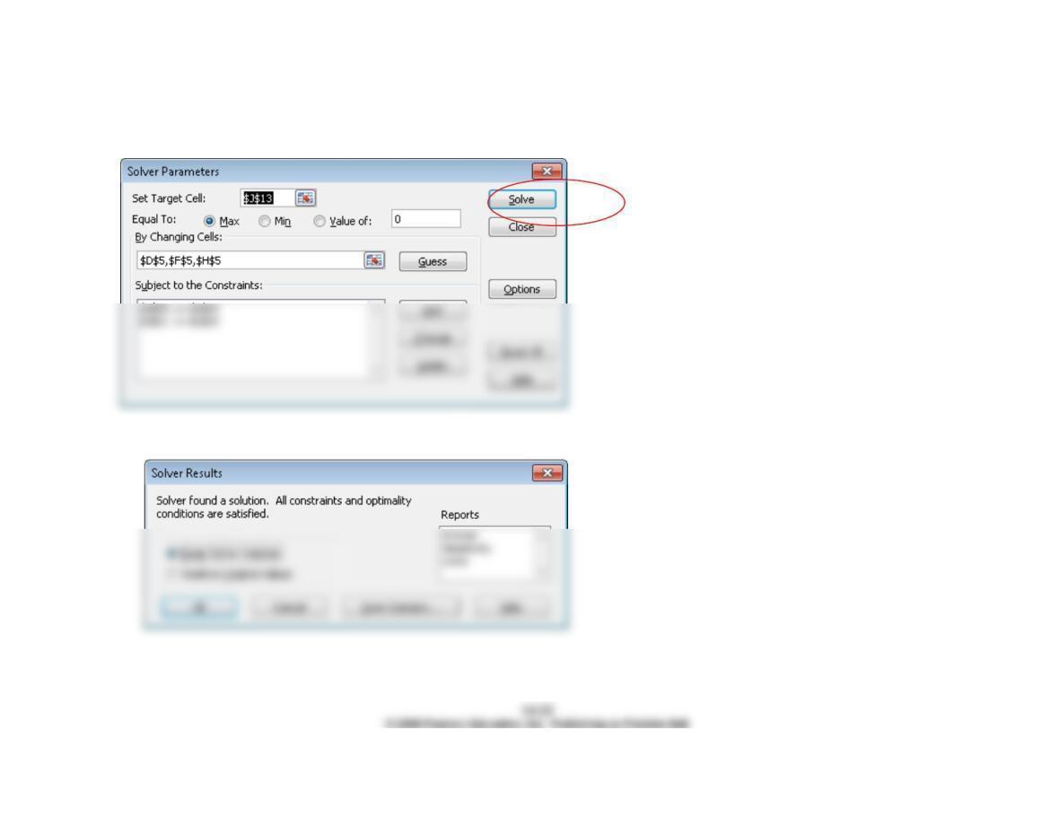
3. Choose “Keep Solver Solution” and click OK
Ch. 14: The Production Cycle
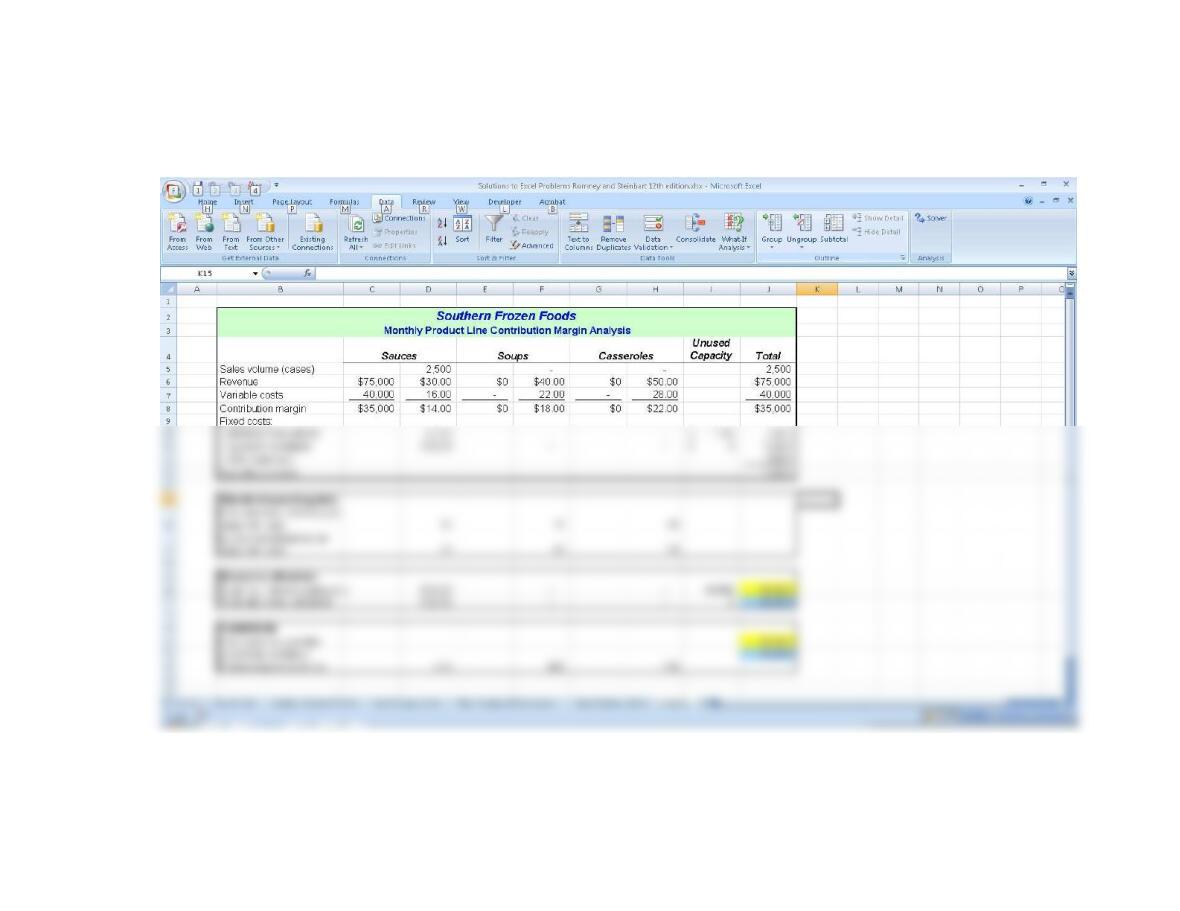
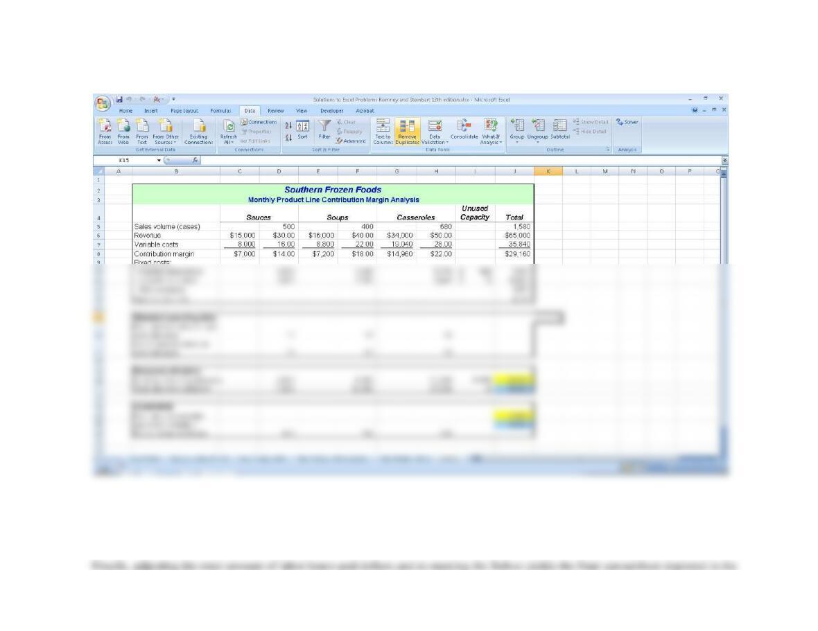
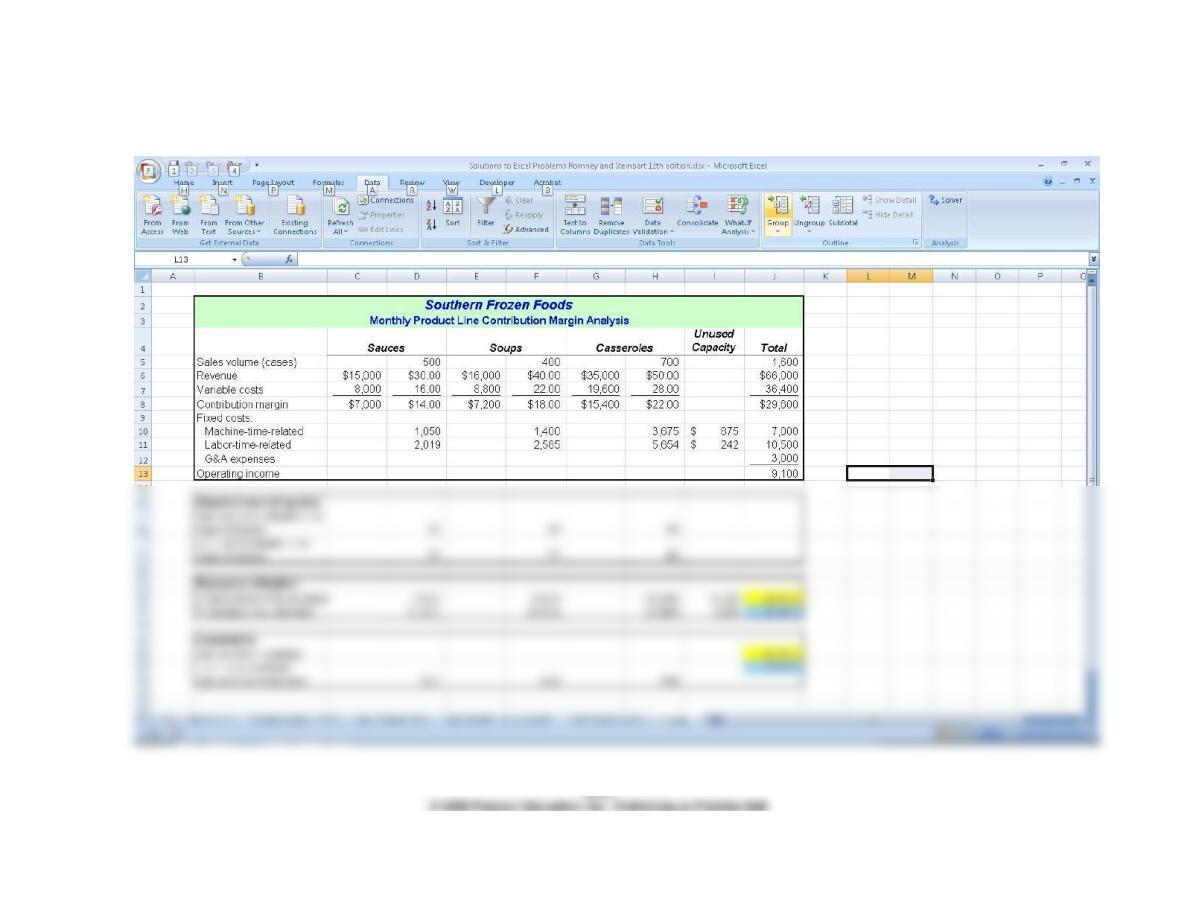
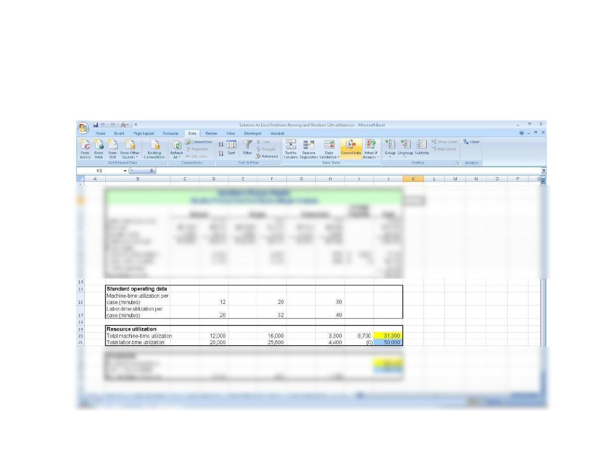
4. The result is the following spreadsheet as shown in the article:
5. Students should save screen shots to show that they have followed the remaining steps in the article.
Production Cycle
Ch. 14: The Production Cycle
Production Cycle
article:
Ch. 14: The Production Cycle
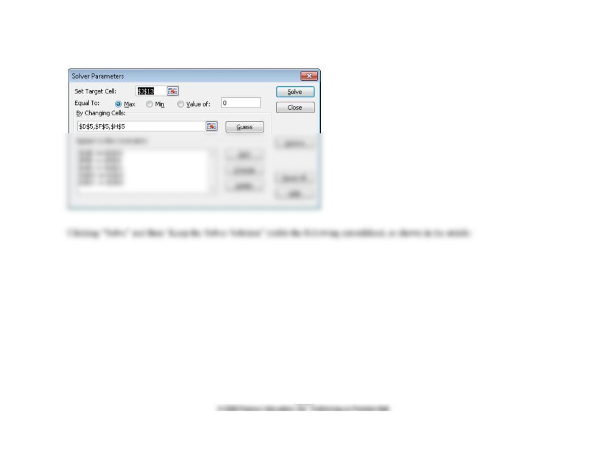
c. Rerun the Solver program to determine the effect of the following actions on income (print out the results of each
option):
• double market share limitations for all three products
Production Cycle
• Double market share limitations for all three products plus the following constraint: sauce case sales cannot exceed
50% of the sum of soup and casserole case sales
Ch. 14: The Production Cycle
Production Cycle
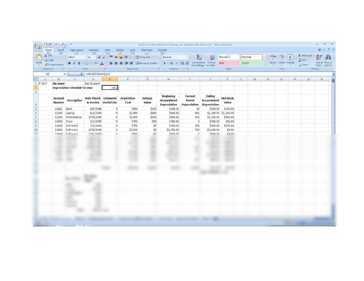
14.9 EXCEL PROBLEM
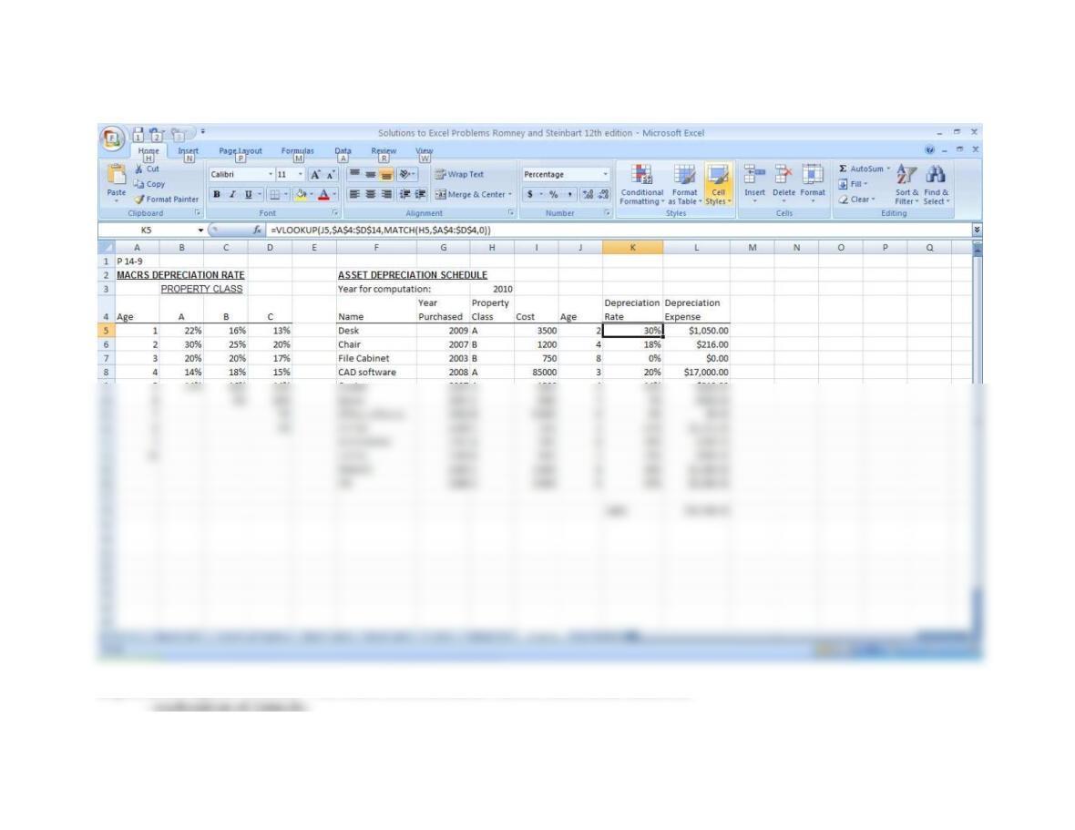
Create the spreadsheet shown in Figure 14-11. Write formulas to calculate the total depreciation expense and to display
Solution is on next page:
Ch. 14: The Production Cycle
Depreciation expense formula: =VLOOKUP(J5,$A$4:$D$14,MATCH(H5,$A$4:$D$4,0))
• The age column subtracts the year the asset was purchased from the reference year in cell H3.
It then adds one to that value because the year the asset is purchased is its first year of
depreciation.
SUGGESTED ANSWERS TO THE CASES
CASE 14-1 The Accountant and CIM
Examine issues of the Journal of Accountancy, Strategic Finance, and other business
magazines for the past three years to find stories about current developments in factory
automation. Write a brief report that discusses the accounting implications of one