Accounting Chapter 13 Homework Vertex baldness and MI after adjusting for age

CHAPTER 13/DESIGN AND ANALYSIS TECHNIQUES FOR EPIDEMIOLOGIC STUDIES 397

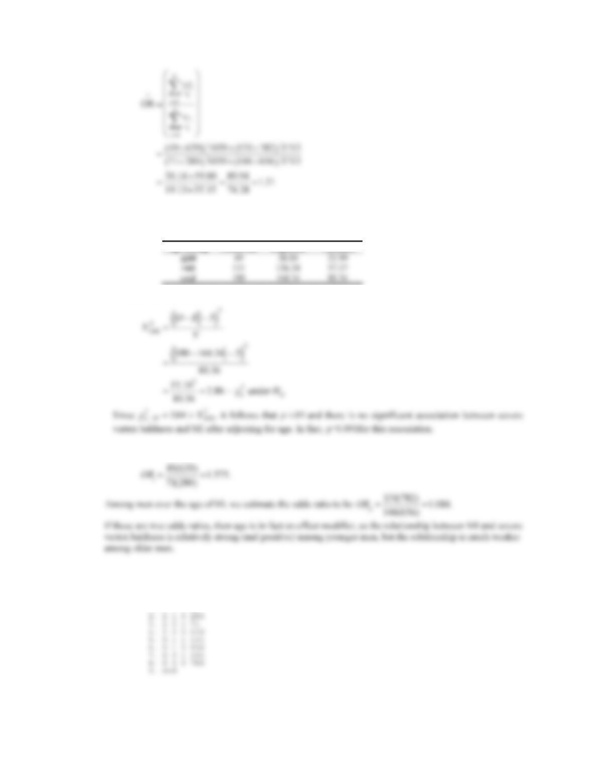
13.95 We now compute the observed (O) and expected (E) number of men in the (1, 1) cell of each table and

the variance of

O

E





.

Age Group Observed Expected Variance

We have the test statistic

13.96 Among men age 60 or under, we estimate the odds ratio between MI and severe vertex baldness as

13.97 To fit our logistic regression models, we enter the following data into STATA.

. input age baldness MI count

age baldness MI count

1. 1 1 1 49

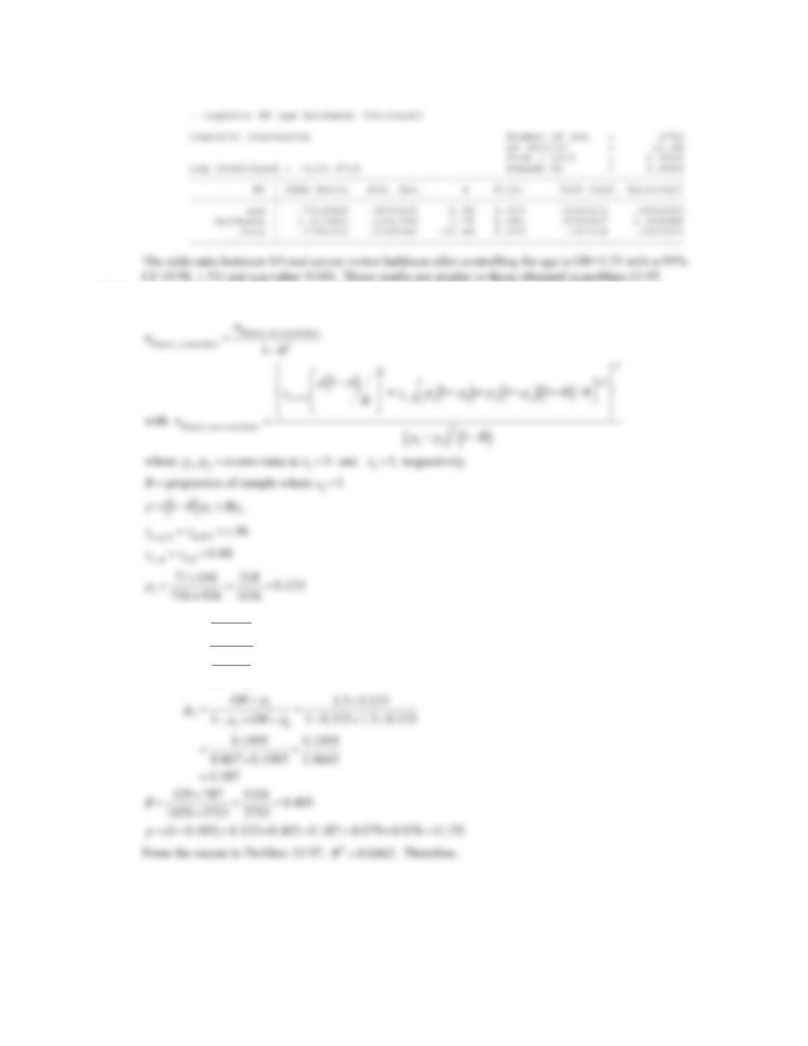
We then fit the logistic regression model as

CHAPTER 13/DESIGN AND ANALYSIS TECHNIQUES FOR EPIDEMIOLOGIC STUDIES 398

13.98 We use equation 13.44 (from the text) to estimate the sample size. Baldness is a binary variable (severe

vertex or none)

Since OR

p

2

1p

2



p

1

1p

1



1.5,we have

CHAPTER 13/DESIGN AND ANALYSIS TECHNIQUES FOR EPIDEMIOLOGIC STUDIES 399

13.99 Before fitting a longitudinal model in STATA, we have to go through a few coding steps first.

Wald chi2(5) = 47.41

Scale parameter: .1306127 Prob > chi2 = 0.0000

——————————————————————————

creat_ | Coef. Std. Err. z P>|z| [95% Conf. Interval]

————-+—————————————————————-

_Igroup_2 | -.1310275 .0434633 -3.01 0.003 -.2162139 -.045841

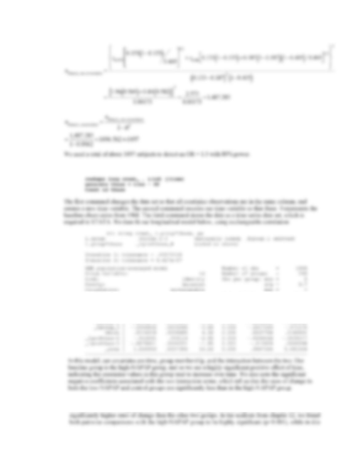
13.100 These findings are qualitatively similar to those in 12.49, in that we found the rate of change in serum-

creatinine levels to be significantly different between groups, with the high-NAPAP group found to have

CHAPTER 13/DESIGN AND ANALYSIS TECHNIQUES FOR EPIDEMIOLOGIC STUDIES 400

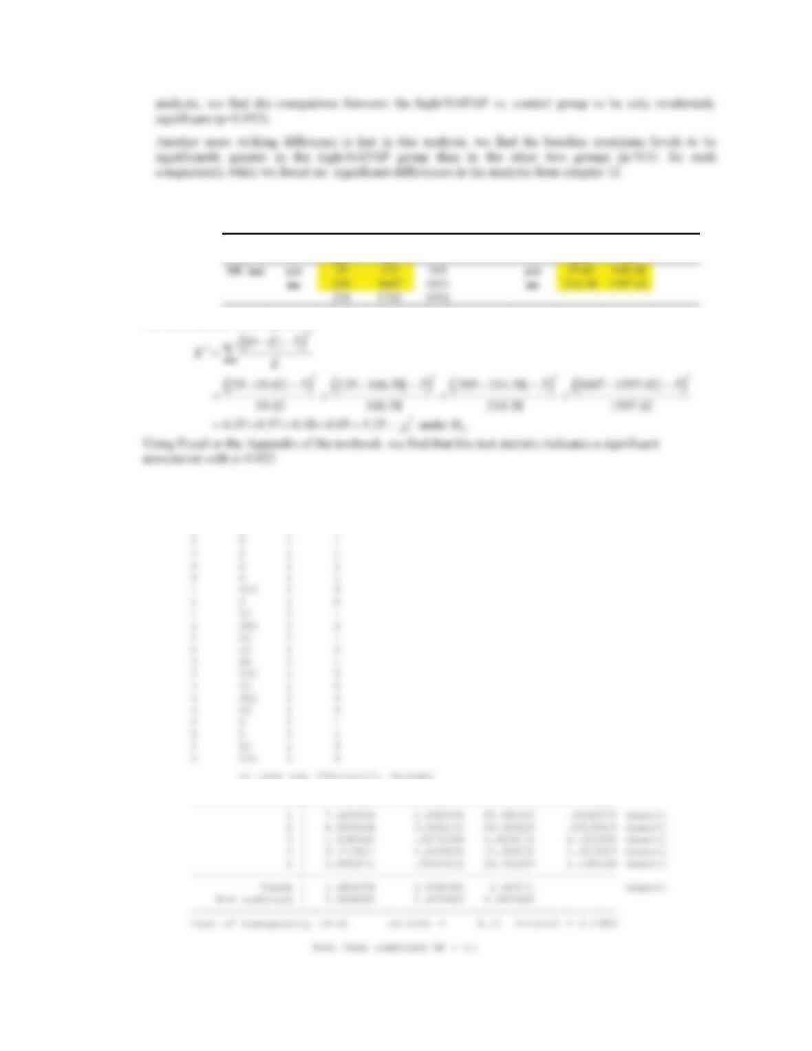
13.101 In Table 13.7, we are given OR=1.7. We can easily calculate the expected and observed counts for each

cell, and then perform a continuity-corrected Chi-Square test.

Ǥ MI Exp. MI

yes no yes no

Our test statistic is then given by

13.102-13.104

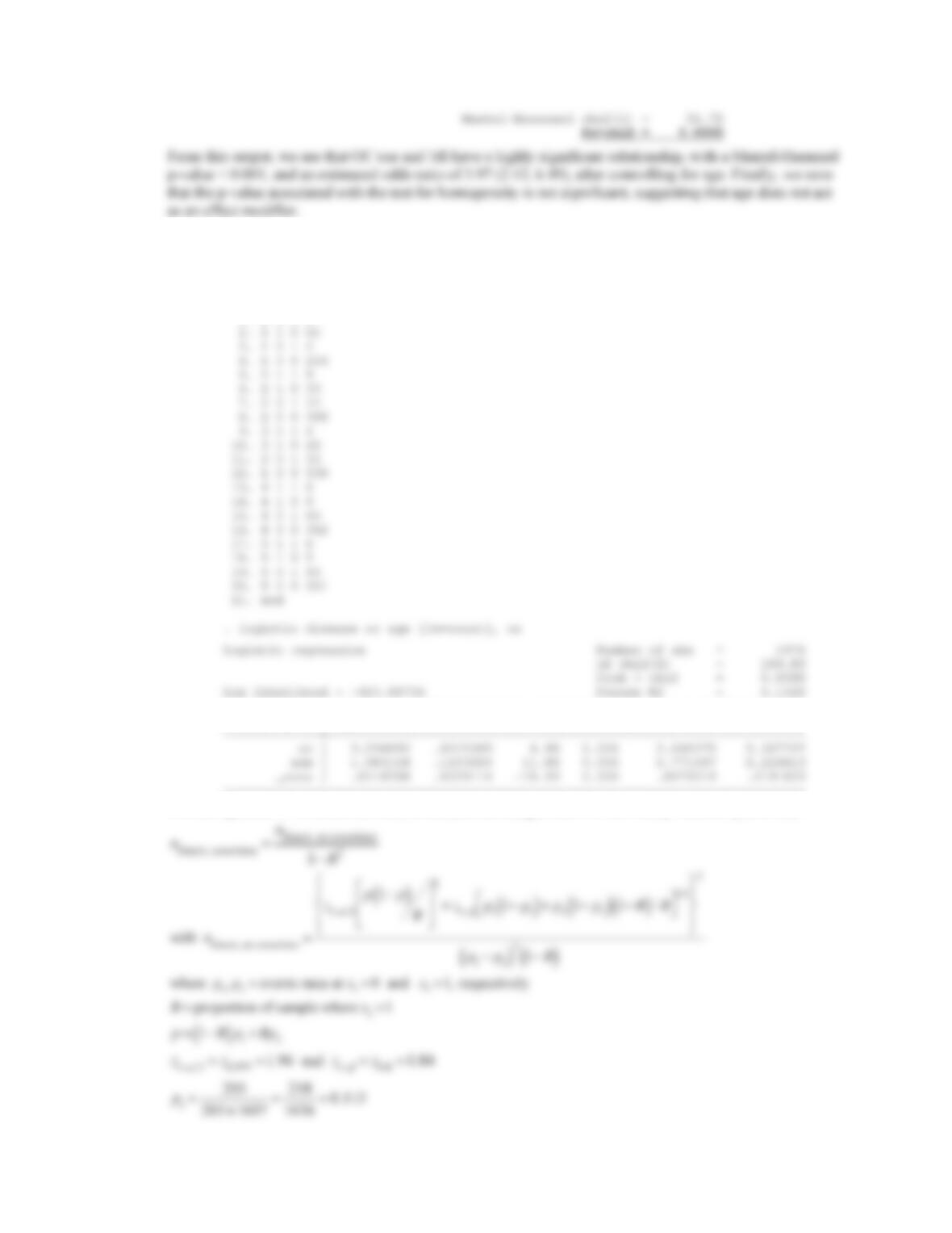
We can use STATA to answer all three of these questions simultaneously. We enter the following data.

age count case exp

1 4 1 1

age | OR [95% Conf. Interval] M-H Weight

CHAPTER 13/DESIGN AND ANALYSIS TECHNIQUES FOR EPIDEMIOLOGIC STUDIES 401

13.105 To fit our logistic regression models, we enter the following data into STATA.

. input age oc disease count

age oc disease count

1. 1 1 1 4

——————————————————————————

disease | Odds Ratio Std. Err. z P>|z| [95% Conf. Interval]

——————————————————————————

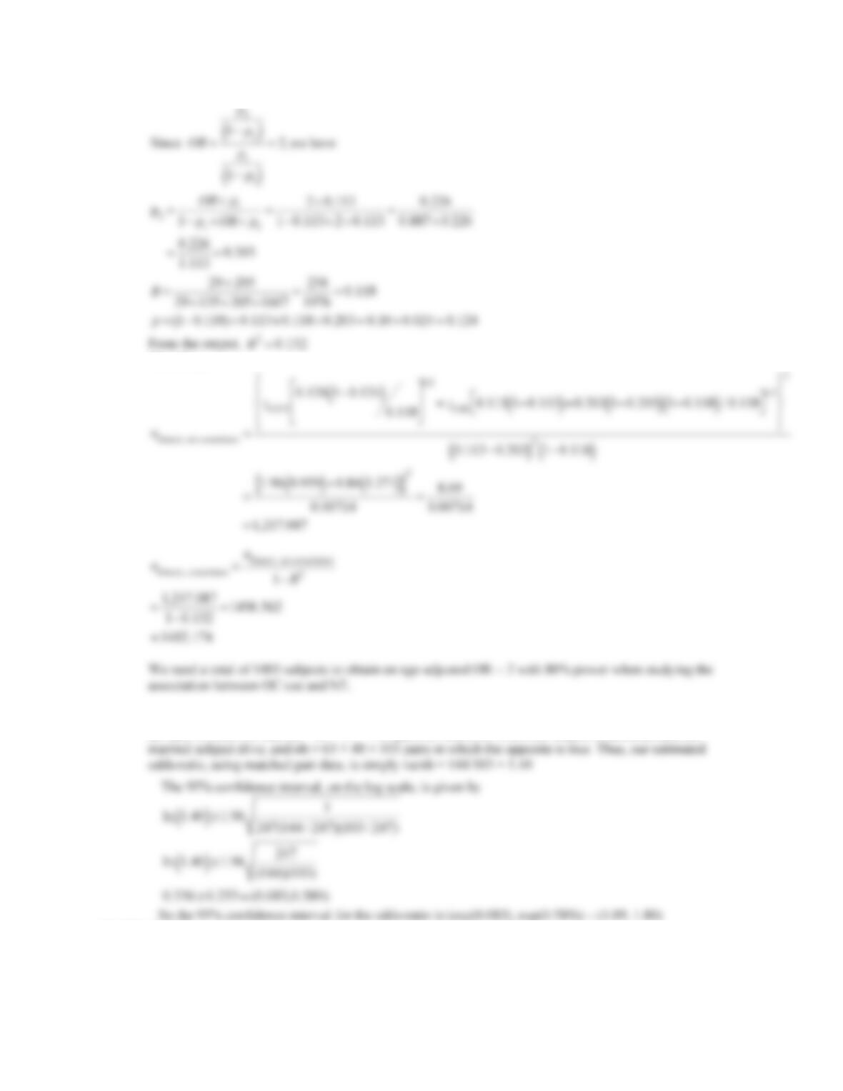
We use equation 13.44 (from the text) to estimate the sample size. OC is a binary variable (yes or no)

CHAPTER 13/DESIGN AND ANALYSIS TECHNIQUES FOR EPIDEMIOLOGIC STUDIES 402

Therefore,

13.106 Due to the low counts found in some of the strata, we choose to estimate the overall odds-ratio, pooling

all data. In total, we find na = 87 + 57 = 144 pairs in which the widowed subject is deceased and the

13.107-13.108

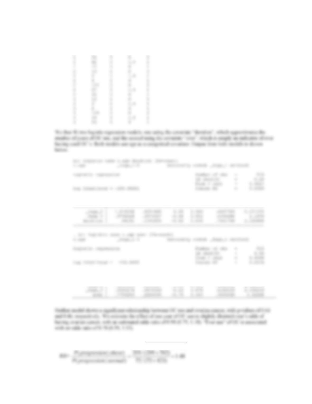
To fit our logistic regression models, we enter the following data into STATA.

CHAPTER 13/DESIGN AND ANALYSIS TECHNIQUES FOR EPIDEMIOLOGIC STUDIES 403

age count case duration ever

1 9 1 0 0

1 2 1 1.5 1

1 0 1 4 1

——————————————————————————

case | Odds Ratio Std. Err. z P>|z| [95% Conf. Interval]

——————————————————————————

case | Odds Ratio Std. Err. z P>|z| [95% Conf. Interval]

————-+—————————————————————-

13.109 We will use Eq. 13.12 with p = P(obesity) = 209 762 0.662

209 762 72 423



 and

CHAPTER 13/DESIGN AND ANALYSIS TECHNIQUES FOR EPIDEMIOLOGIC STUDIES 404

13.110 The 95% CI is given by

e

c1

1e

c1

,e

c2

1e

c2

§

©

¨

·

¹

¸,

where

13.111-13.112 We enter the following data into STATA.

age count aspirin cvd

1 163 1 1

1 11847 1 0

1 161 0 1

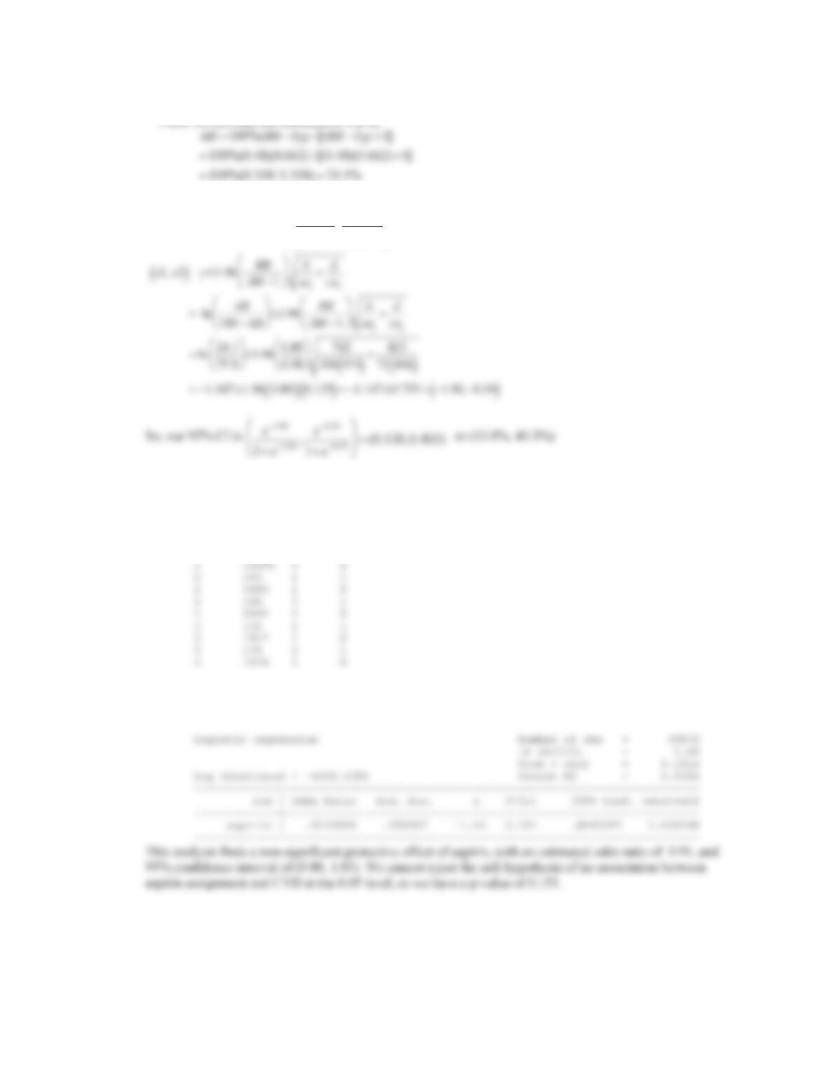
Our first model only uses a single covariate, the indicator of aspirin usage.

logistic cvd aspirin [fw=count]

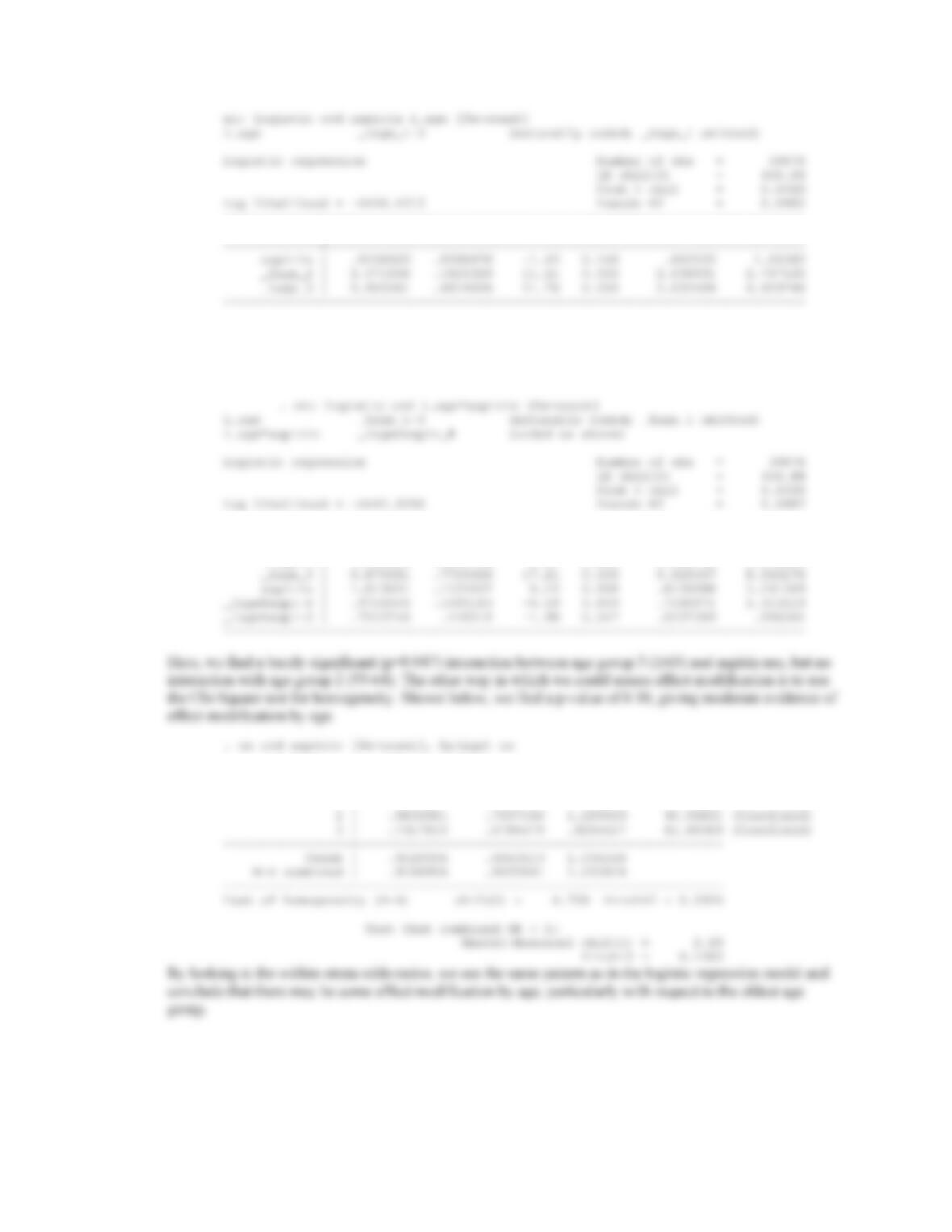
13.113 Though we find age to have a highly significant relationship with CVD, we find little to no evidence of

confounding by age. Our new model, which controls for age using indicator variables for each age group,

estimates the effect of aspirin to be nearly unchanged, with estimated OR = 0.91(0.80, 1.03).

CHAPTER 13/DESIGN AND ANALYSIS TECHNIQUES FOR EPIDEMIOLOGIC STUDIES 405

——————————————————————————

cvd | Odds Ratio Std. Err. z P>|z| [95% Conf. Interval]

13.114 We can attempt to assess effect modification in two ways. The first is to fit a logistic regression model

which contains interaction effects between the categorical age covariate and the indicator of aspirin use.

The results from this model are shown below.

——————————————————————————

cvd | Odds Ratio Std. Err. z P>|z| [95% Conf. Interval]

————-+—————————————————————-

_Iage_2 | 2.405953 .2618796 8.07 0.000 1.943734 2.978087

age | OR [95% Conf. Interval] M-H Weight

—————–+————————————————-

1 | 1.013021 .8139101 1.26084 79.39093 (Cornfield)

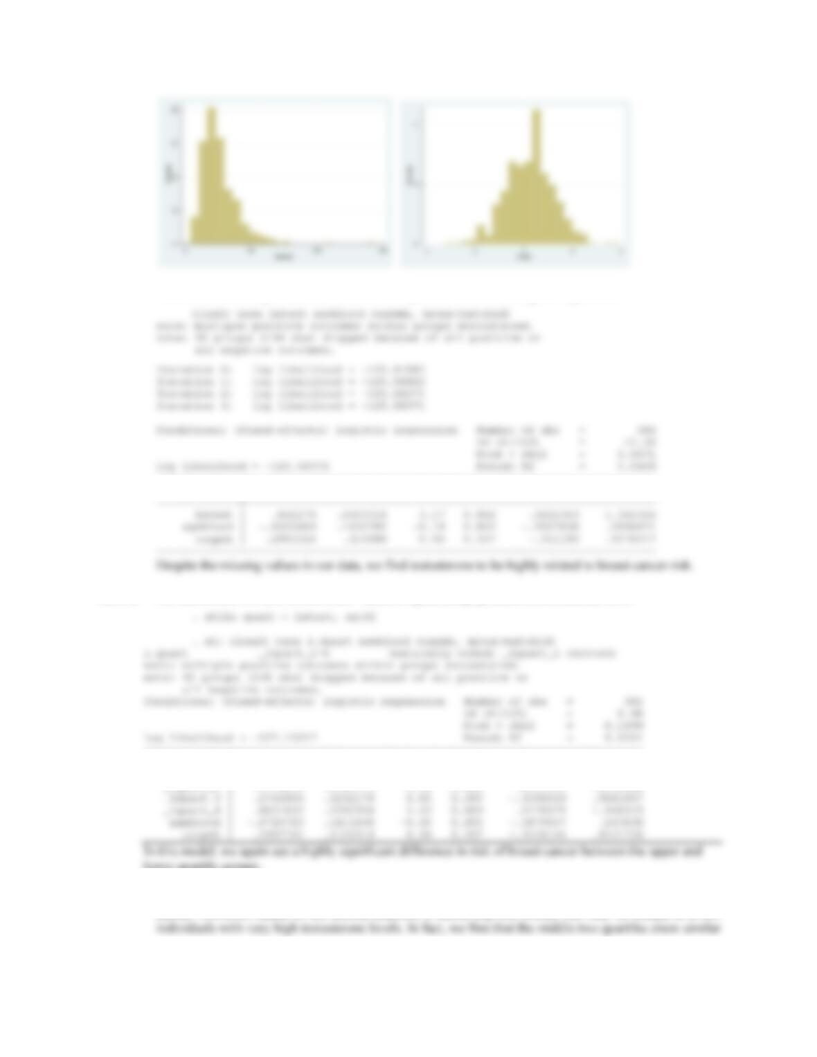
13.115 First, we examine the distribution of the variable “testost”, and decide to use a ln- transformation to make

the variable somewhat more normally distributed.

CHAPTER 13/DESIGN AND ANALYSIS TECHNIQUES FOR EPIDEMIOLOGIC STUDIES 406

Next we use the clogit command in STATA to perform conditional logistic regression.

——————————————————————————

case | Coef. Std. Err. z P>|z| [95% Conf. Interval]

13.116 For this model, we must create a new variable representing quartiles of testosterone level.

——————————————————————————

case | Coef. Std. Err. z P>|z| [95% Conf. Interval]

————-+—————————————————————-

_Iquart_2 | .2116893 .3183474 0.66 0.506 -.4122601 .8356388

lower quartile groups..

13.117 Based on the previous two questions, it seems that testosterone levels are clearly related to risk of breast

cancer. However, based on the second analysis, it seems that this excess risk may be related to a few

CHAPTER 13/DESIGN AND ANALYSIS TECHNIQUES FOR EPIDEMIOLOGIC STUDIES 407

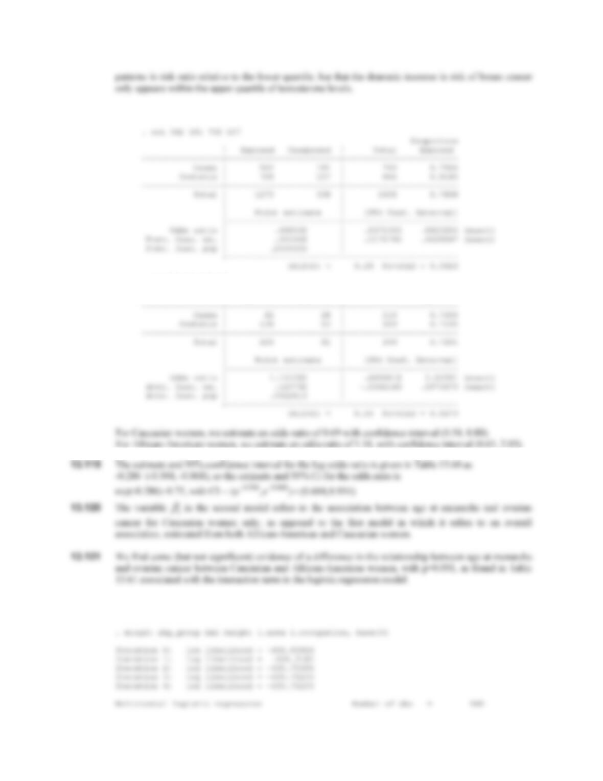
13.118 We can use the cci command in STATA to calculate these odds-ratios directly.

. cci 82 28 136 53

Proportion

| Exposed Unexposed | Total Exposed

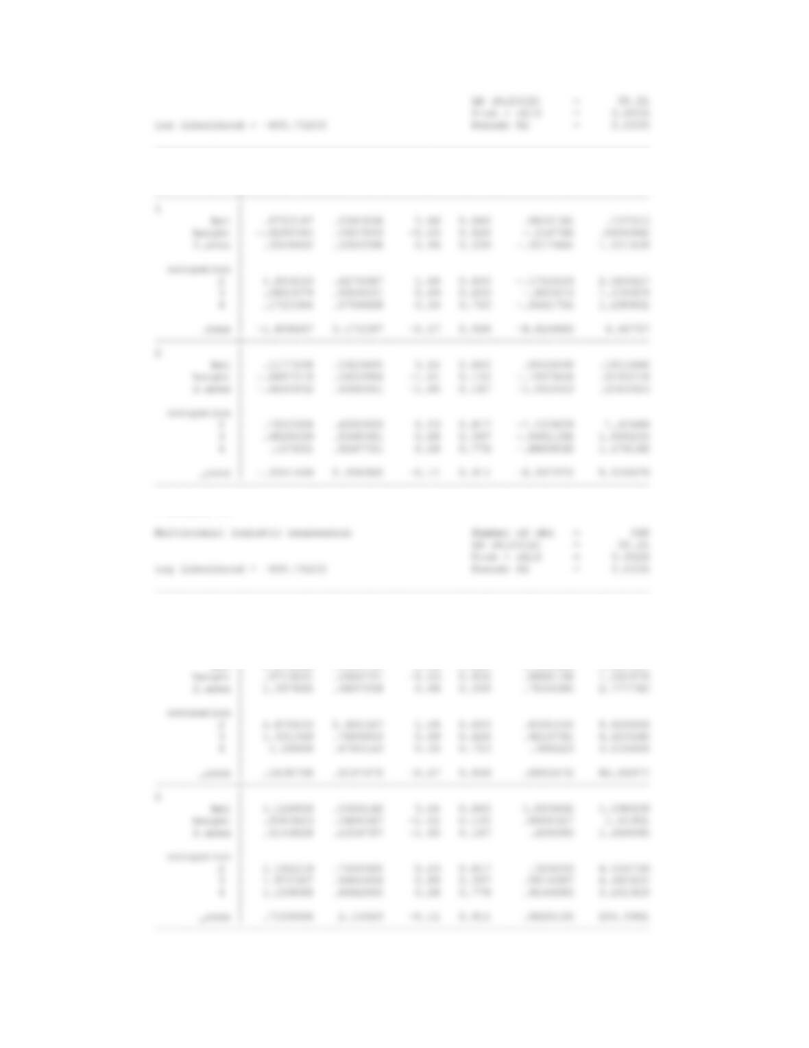
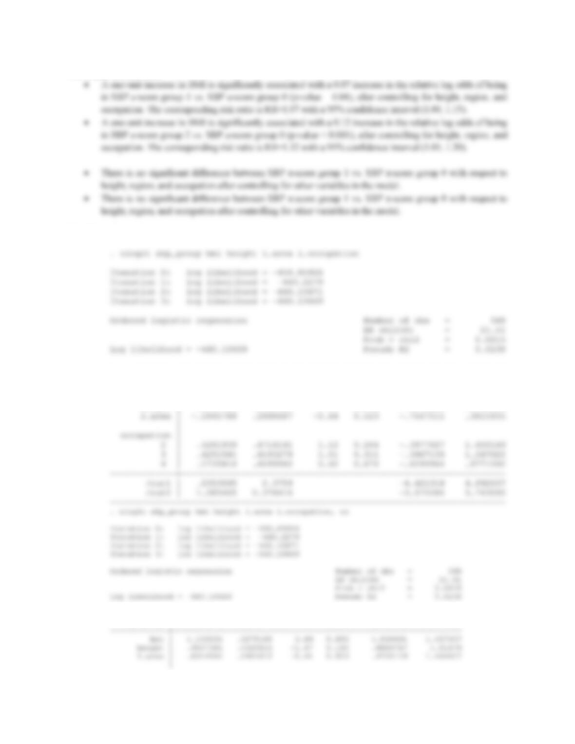
13.122 We run polytomous logistic regression for SBP z-score group in Stata and generate the corresponding

risk ratio table below:

CHAPTER 13/DESIGN AND ANALYSIS TECHNIQUES FOR EPIDEMIOLOGIC STUDIES 408

——————————————————————————

sbp_group | Coef. Std. Err. z P>|z| [95% Conf. Interval]

————-+—————————————————————-

0 | (base outcome)

. mlogit, rr

——————————————————————————

sbp_group | RRR Std. Err. z P>|z| [95% Conf. Interval]

————-+—————————————————————-

0 | (base outcome)

————-+—————————————————————-

1 |

bmi | 1.072846 .0366735 2.06 0.040 1.003322 1.147187

CHAPTER 13/DESIGN AND ANALYSIS TECHNIQUES FOR EPIDEMIOLOGIC STUDIES 409

The output indicates that:

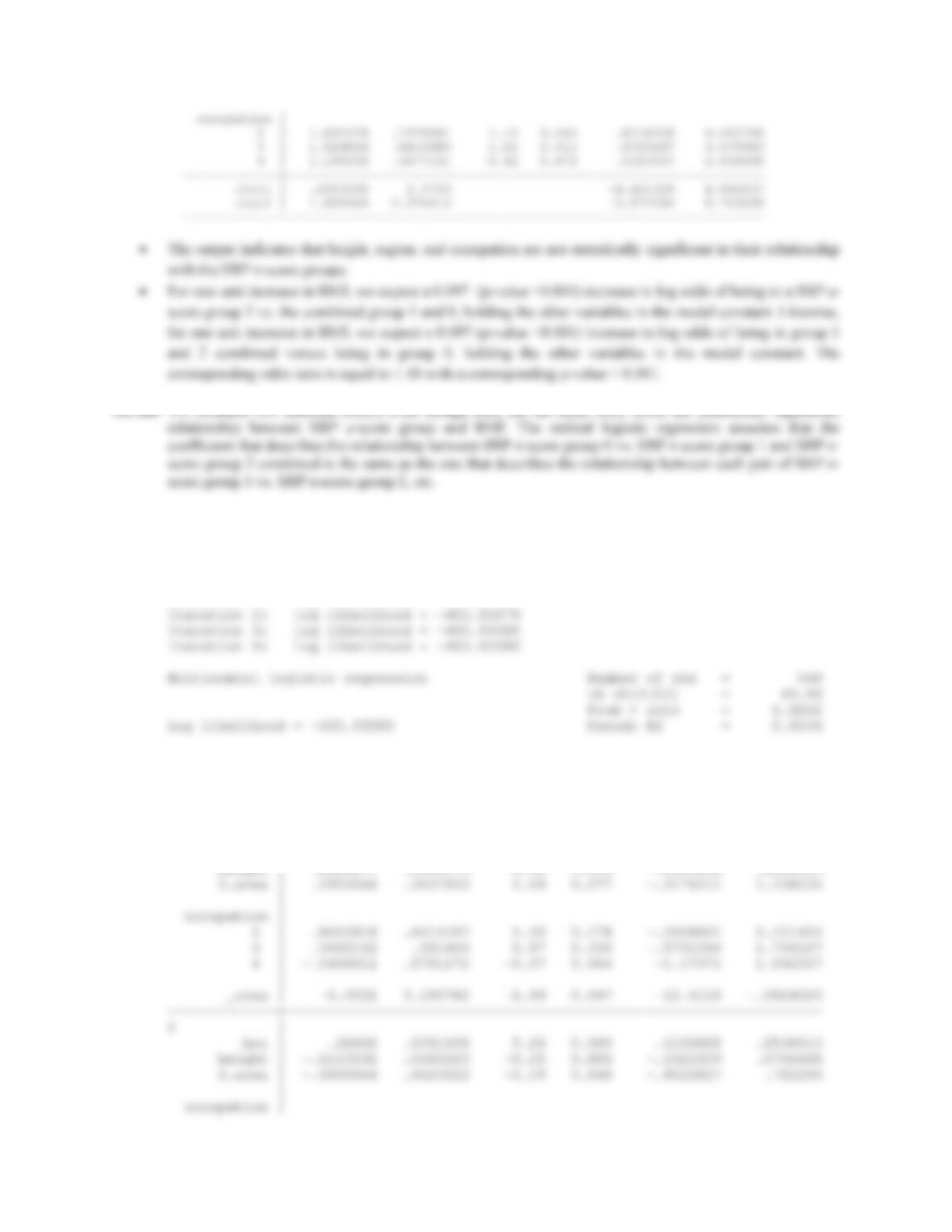
13.123 The ordinal logistic regression for SBP z-score group variable gives the following results:

——————————————————————————

sbp_group | Coef. Std. Err. z P>|z| [95% Conf. Interval]

————-+—————————————————————-

bmi | .0971579 .0249688 3.89 0.000 .0482198 .1460959

height | -.0505166 .0342698 -1.47 0.140 -.1176842 .0166509

——————————————————————————

sbp_group | Odds Ratio Std. Err. z P>|z| [95% Conf. Interval]

CHAPTER 13/DESIGN AND ANALYSIS TECHNIQUES FOR EPIDEMIOLOGIC STUDIES 410

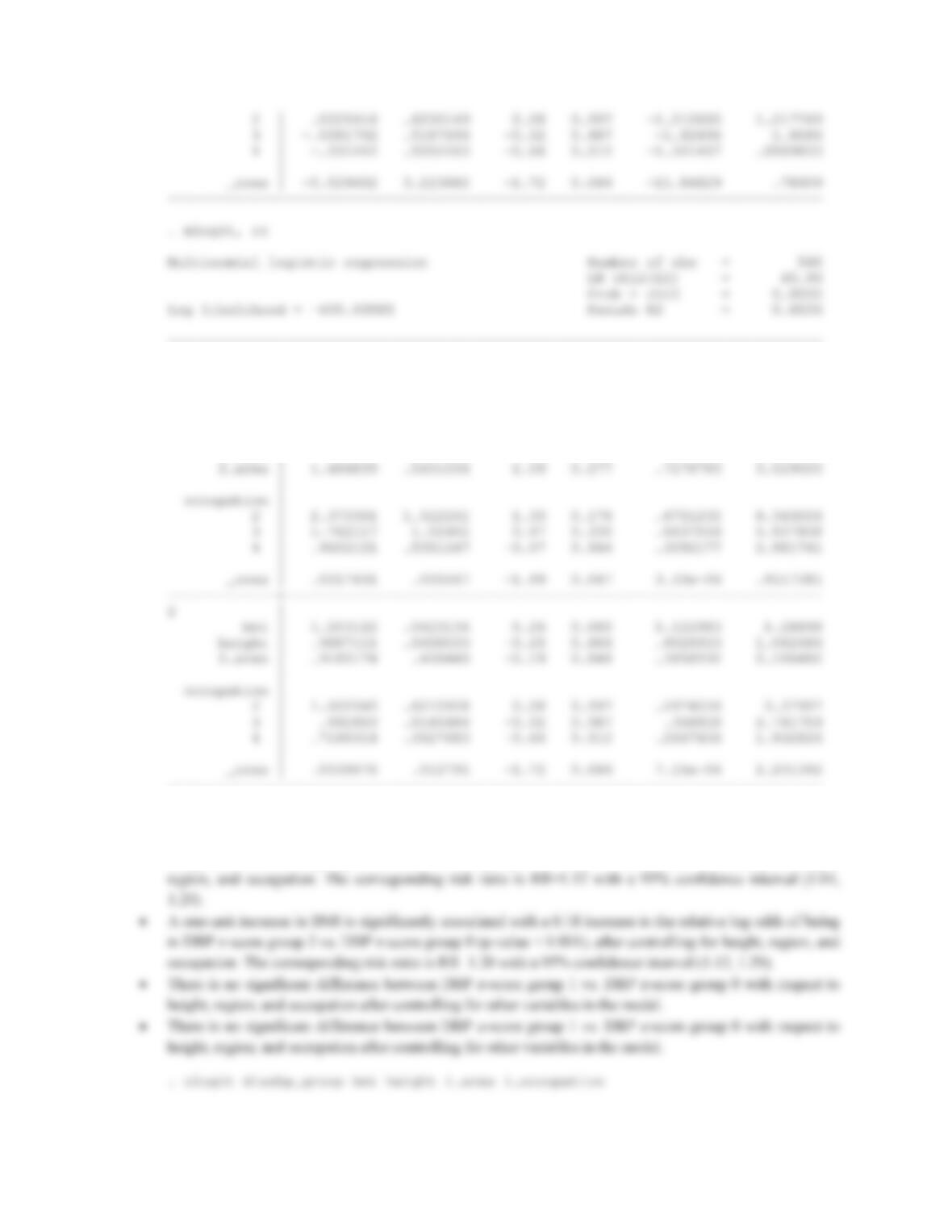
13.125 For diastolic blood pressure we have the following results:

. mlogit diasbp_group bmi height i.area i.occupation, base(0)

Iteration 0: log likelihood = -428.9142

Iteration 1: log likelihood = -406.57283

——————————————————————————

diasbp_group | Coef. Std. Err. z P>|z| [95% Conf. Interval]

————-+—————————————————————-

0 | (base outcome)

————-+—————————————————————-

1 |

bmi | .1128247 .0348918 3.23 0.001 .0444381 .1812113

CHAPTER 13/DESIGN AND ANALYSIS TECHNIQUES FOR EPIDEMIOLOGIC STUDIES 411

——————————————————————————

diasbp_group | RRR Std. Err. z P>|z| [95% Conf. Interval]

————-+—————————————————————-

0 | (base outcome)

————-+—————————————————————-

1 |

bmi | 1.119436 .0390591 3.23 0.001 1.04544 1.198668

height | 1.02309 .0465689 0.50 0.616 .9357698 1.118559

——————————————————————————

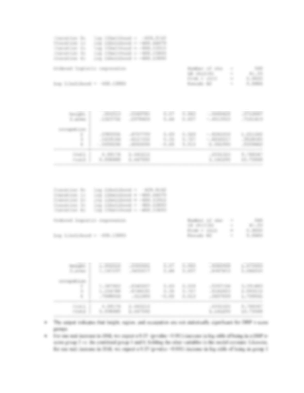
The output indicates that:

xA one-unit increase in BMI is significantly associated with a 0.113 increase in the relative log odds of

being in DBP z-score group 1 vs. DBP z-score group 0 (p-value = 0.001), after controlling for height,

CHAPTER 13/DESIGN AND ANALYSIS TECHNIQUES FOR EPIDEMIOLOGIC STUDIES 412

——————————————————————————

diasbp_group | Coef. Std. Err. z P>|z| [95% Conf. Interval]

————-+—————————————————————-

bmi | .1517988 .0266264 5.70 0.000 .0996122 .2039855

. ologit diasbp_group bmi height i.area i.occupation, or

——————————————————————————

diasbp_group | Odds Ratio Std. Err. z P>|z| [95% Conf. Interval]

————-+—————————————————————-

bmi | 1.163926 .0309911 5.70 0.000 1.104742 1.22628

CHAPTER 13/DESIGN AND ANALYSIS TECHNIQUES FOR EPIDEMIOLOGIC STUDIES 413