Accounting Chapter 13 Homework The difference in previous IUD usage rates is highly

359

=

DESIGN AND ANALYSIS

TECHNIQUES FO

R

EPIDEMIOLOGIC STUDIES

13.1 We wish to test the hypothesis

H

pp

H

pp

01 2 11 2

::, zversus where p1 Pr (infertile woman had ever

used an IUD), p2 Pr (fertile woman had ever used an IUD). We have the test statistic

13.2 We first construct the observed table as follows

ever IUD use

yes no

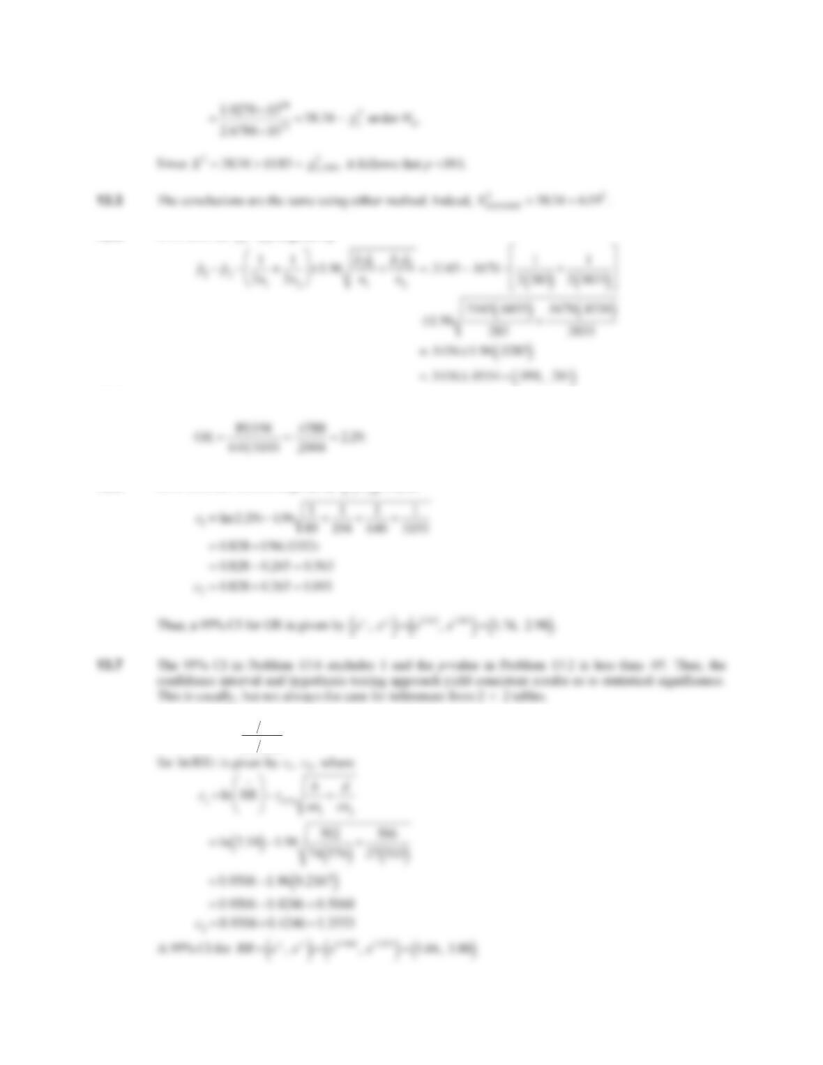
We then compute the chi-square statistic using the short computational form as follows

CHAPTER 13/DESIGN AND ANALYSIS TECHNIQUES FOR EPIDEMIOLOGIC STUDIES 360

13.4 A 95% CI for pp

 is given by

13.5 We have

13.6 A 95% CI for ln OR



is given by

c1,c2



, where

13.8 The risk ratio

74 576

27 533 254.. We use Equation 13.6 to obtain 95% confidence limits for RR. A 95% CI

CHAPTER 13/DESIGN AND ANALYSIS TECHNIQUES FOR EPIDEMIOLOGIC STUDIES 361

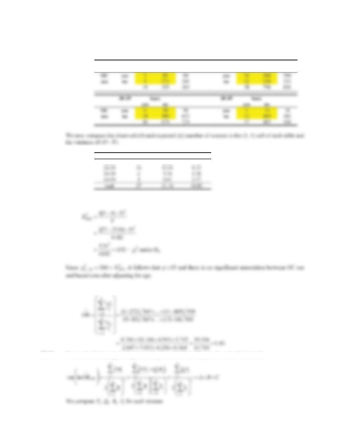
13.9 We will use the Mantel-Haenszel test. We construct 2 u 2 tables relating OC use and bacteriuria for each

age group

16-19 bact. 20-29 bact.

yes no yes no

Age Group Observed Expected Variance

16-19 1 2.30 1.73

We have the test statistic

13.10 The Mantel-Haenszel odds ratio estimate is given by

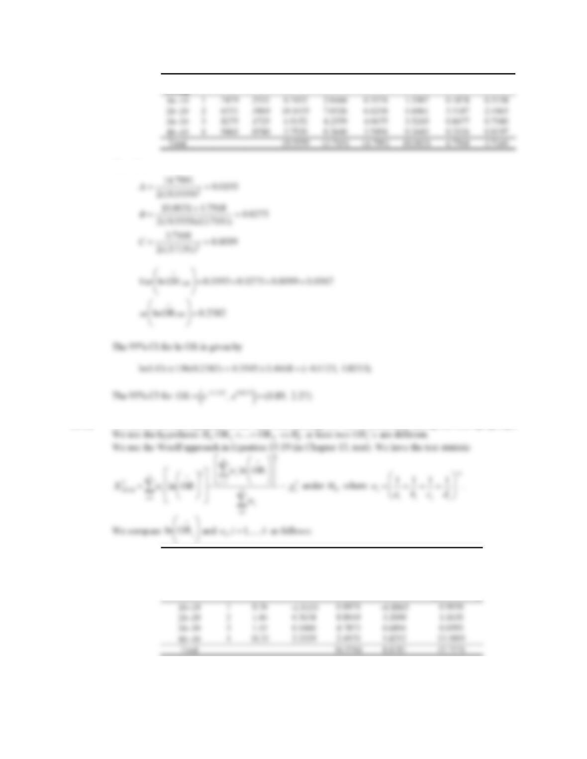
13.11 We use the Robins approach given in Equation 13.18 (in Chapter 13, text). We have that

CHAPTER 13/DESIGN AND ANALYSIS TECHNIQUES FOR EPIDEMIOLOGIC STUDIES 362

Age

Group

iP

i

Q

i

R

iSi

P

R

ii

P

S

ii Q

R

ii

Q

S

ii

Therefore,

13.12 We test for the heterogeneity of the odds ratio relating OC use to bacteriuria among the four age groups.

Age Group iOR

^

i

ln ORi



§

©

¨

·

¹

¸

w

i

wiln ORi



§

©

¨

·

¹

¸

wiln ORi



§

©

¨

·

¹

¸

2

ª

¬

«

º

¼

»

We have

CHAPTER 13/DESIGN AND ANALYSIS TECHNIQUES FOR EPIDEMIOLOGIC STUDIES 363

13.13 We form a single 2 u 2 table pooling all the age-specific tables together. We have

bacteriuria

yes no

13.14 Interestingly, the crude and adjusted odds ratios are virtually the same in these data. Bacteriuria rates

13.16 We have the test statistic

Thus,

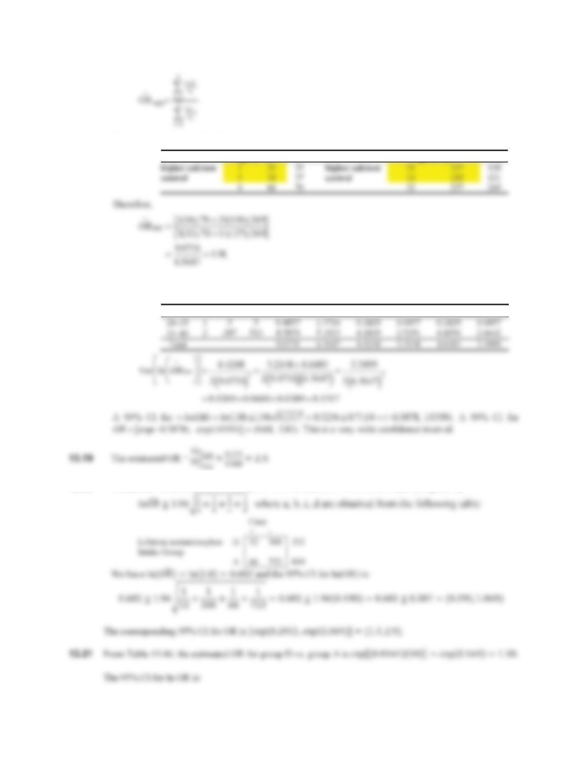
13.17 We use the Mantel-Haenszel odds ratio estimate as follows:

CHAPTER 13/DESIGN AND ANALYSIS TECHNIQUES FOR EPIDEMIOLOGIC STUDIES 364

We have the following 2 u 2 tables:

age 20



35 age 5580

13.18 We use the Robins approach given in Equation 13.18 (in Chapter 13, text). Thus, we have the following

summary statistics:

group iP

i

Q

i

R

iSi

P

R

ii

P

S

ii Q

R

ii

Q

S

ii

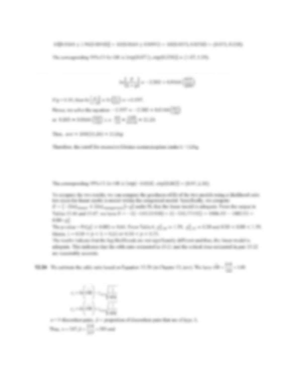
13.20 We use the Woolf formula to obtain a 95% CI for the OR. A 95% CI for ln(OR) is given by:

CHAPTER 13/DESIGN AND ANALYSIS TECHNIQUES FOR EPIDEMIOLOGIC STUDIES 365

13.22 We wish to find a level of ace/100 such that p = 0.10. From the logistic regression, we have:

13.23 From Table 13.47, the estimated OR for group C versus group A is given by ሾሺͲǤͶʹ͵ሻሿൌͳǤͷ͵.

The 95% CI for ln OR is: ሾͲǤͶʹ͵േͳǤͻ͸ሺͲǤʹʹ͵ሻሿൌሺെͲǤͲͳͶǡͲǤͺ͸ሻ.

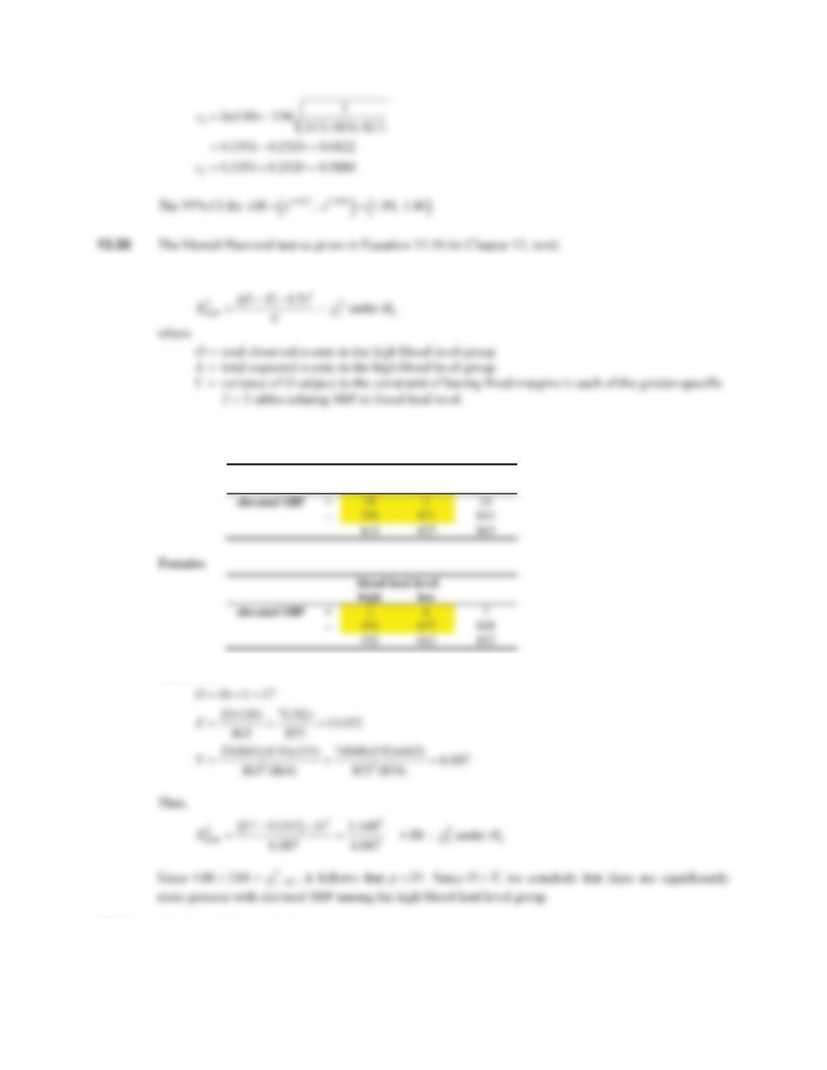
13.25 A 95% CI for

OR e

c

1

,e

c

2



, where

CHAPTER 13/DESIGN AND ANALYSIS TECHNIQUES FOR EPIDEMIOLOGIC STUDIES 366

13.27 We have the test statistic

We have the following 2 u 2 tables by gender:

Males

blood lead level

high low

Therefore,

13.28 The Mantel-Haenszel odds ratio is given by

CHAPTER 13/DESIGN AND ANALYSIS TECHNIQUES FOR EPIDEMIOLOGIC STUDIES 367

gender iP

i

Q

i

R

iSi

P

R

ii

P

S

ii Q

R

ii

Q

S

ii

We have

13.29 To address this question, we can use STATA’s powerful metan command, which performs both fixed-

effects and random-effects meta-analyses of 2×2 tables. We must first reshape the data so that each trial

CHAPTER 13/DESIGN AND ANALYSIS TECHNIQUES FOR EPIDEMIOLOGIC STUDIES 368

Study | OR [95% Conf. Interval] % Weight

CHAPTER 13/DESIGN AND ANALYSIS TECHNIQUES FOR EPIDEMIOLOGIC STUDIES 369

Study | OR [95% Conf. Interval] % Weight

(27 missing values generated)

Study | OR [95% Conf. Interval] % Weight

CHAPTER 13/DESIGN AND ANALYSIS TECHNIQUES FOR EPIDEMIOLOGIC STUDIES 370

Study | OR [95% Conf. Interval] % Weight

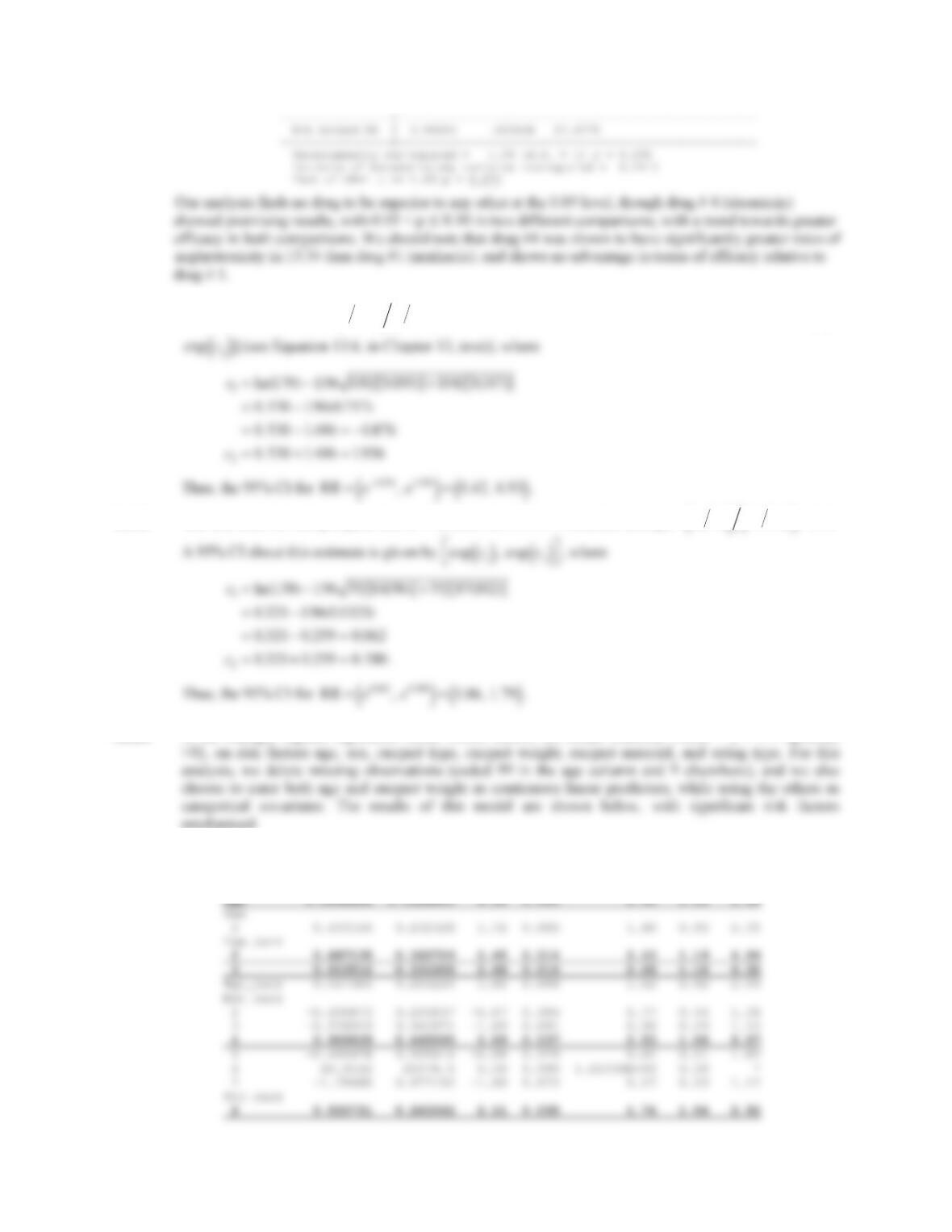
13.30 We use the same procedure as in Problem 13.29, but this time we note that we only have sufficient data

for drug 4 to compare it with drug 2. All other pairwise comparisons are made, with significant results

emphasized.

. metan side_eff1 noside1 side_eff2 noside2, or fixedi nograph

(16 missing values generated)

Study | OR [95% Conf. Interval] % Weight

—————–+——————————————————-

1 | 1.59615 .750004 3.39692 54.5655

Study | OR [95% Conf. Interval] % Weight

—————–+——————————————————-

3 | .492063 .018238 13.2757 14.4067

CHAPTER 13/DESIGN AND ANALYSIS TECHNIQUES FOR EPIDEMIOLOGIC STUDIES 371

Study | OR [95% Conf. Interval] % Weight

—————–+——————————————————-

3 | .28 .008952 8.75782 13.3031

(16 missing values generated)

Study | OR [95% Conf. Interval] % Weight

—————–+——————————————————-

1 | .407407 .013135 12.6365 12.2534

Study | OR [95% Conf. Interval] % Weight

—————–+——————————————————-

14 | .317073 .012171 8.26047 15.3373

Study | OR [95% Conf. Interval] % Weight

—————–+——————————————————-

1 | .317073 .012171 8.26047 15.3373

Study | OR [95% Conf. Interval] % Weight

—————–+——————————————————-

5 | .155556 .0055 4.39958 11.7644

CHAPTER 13/DESIGN AND ANALYSIS TECHNIQUES FOR EPIDEMIOLOGIC STUDIES 372

Study | OR [95% Conf. Interval] % Weight

13.31 We again repeat the procedure from 13.29 and 13.30, noting that there is insufficient data to compare the

efficacy of drug 3 vs. 4. All other comparisons are shown below.

reshape wide samp_sz cured, i(id) j(antibio)

(note: j = 1 2 3 4 5)

. metan cured1 nocure1 cured2 nocure2, or fixedi nograph

(21 missing values generated)

Study | OR [95% Conf. Interval] % Weight

—————–+——————————————————-

6 | 1.33333 .300556 5.91496 5.71014

Study | OR [95% Conf. Interval] % Weight

—————–+——————————————————-

4 | .775862 .211995 2.83951 19.1232

Study | OR [95% Conf. Interval] % Weight

CHAPTER 13/DESIGN AND ANALYSIS TECHNIQUES FOR EPIDEMIOLOGIC STUDIES 373

Study | OR [95% Conf. Interval] % Weight

—————–+——————————————————-

Study | OR [95% Conf. Interval] % Weight

—————–+——————————————————-

1 | 3.5 .549235 22.3038 28.8728

Study | OR [95% Conf. Interval] % Weight

—————–+——————————————————-

1 | 1.6 .236849 10.8086 6.07067

4 | 1.72414 .377227 7.88027 9.59352

Study | OR [95% Conf. Interval] % Weight

—————–+——————————————————-

1 | 1.6 .236849 10.8086 6.29411

2 | 1.72414 .377227 7.88027 9.83708

Study | OR [95% Conf. Interval] % Weight

—————–+——————————————————-

11 | 1.01316 .567042 1.81025 48.4649

CHAPTER 13/DESIGN AND ANALYSIS TECHNIQUES FOR EPIDEMIOLOGIC STUDIES 374

. metan cured2 nocure2 cured4 nocure4, or randomi nograph

(23 missing values generated)

Study | OR [95% Conf. Interval] % Weight

—————–+——————————————————-

1 | 1.01316 .567042 1.81025 28.254

2 | .127273 .004606 3.51676 3.67639

Study | OR [95% Conf. Interval] % Weight

—————–+——————————————————-

2 | 4.2 .116076 151.97 1.20805

7 | 3 .459365 19.5923 4.41801

. metan cured3 nocure3 cured5 nocure5, or fixedi nograph

(26 missing values generated)

Study | OR [95% Conf. Interval] % Weight

—————–+——————————————————-

2 | 1.875 .302396 11.6259 10.6108

Study | OR [95% Conf. Interval] % Weight

CHAPTER 13/DESIGN AND ANALYSIS TECHNIQUES FOR EPIDEMIOLOGIC STUDIES 375

13.32 The risk ratio for

MI 5105



3 107



1.70

. A 95% CI about this estimate is given by [

exp c

1



,

13.33 The risk ratio for being angina-free at 6 months for PTCA vs medical therapy

61 96



47 102



1.38

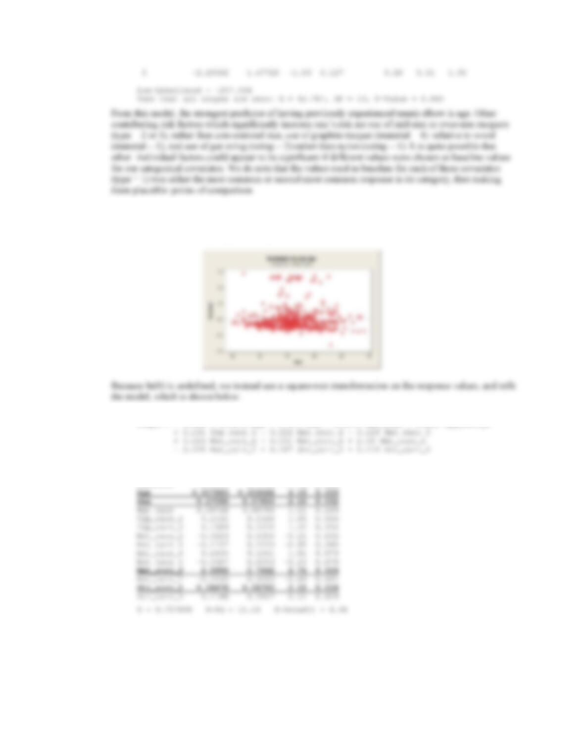
13.34 In the multiple logistic regression model shown below, we model outcome Elbow = { 1 if # episodes

emphasized.

Logistic Regression Table

95% CI

Predictor Coef SE Coef Z P Odds Ratio Lower Upper

Constant -3.35907 0.908135 -3.70 0.000

Age 0.0538286 0.0128859 4.18 0.000 1.06 1.03 1.08

CHAPTER 13/DESIGN AND ANALYSIS TECHNIQUES FOR EPIDEMIOLOGIC STUDIES 376

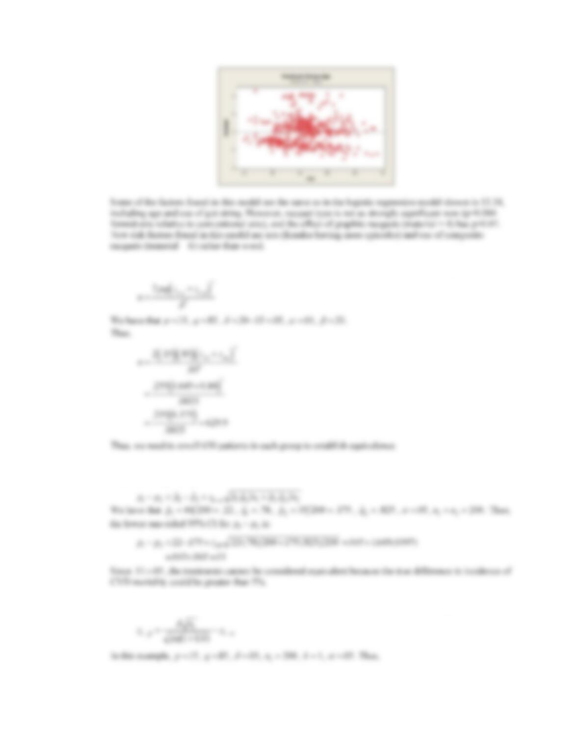
13.35 We first fit a linear regression model using the same factors as above, but using # of episodes as the

outcome variable. However, we find that the residual plot shows that a transformation of the data is

necessary (see “residuals vs. age” below)

The regression equation is

rteps = – 0.552 + 0.0179 Age + 0.170 Sex + 0.0973 Wgt_curr + 0.214 Typ_curr_2

432 cases used, 12 cases contain missing values

Predictor Coef SE Coef T P

Constant -0.5515 0.3140 -1.76 0.080

CHAPTER 13/DESIGN AND ANALYSIS TECHNIQUES FOR EPIDEMIOLOGIC STUDIES 377

13.36 We refer to Equation 13.48 (in Chapter 13, text). The number of patients required in each group is

13.37 We will use the lower one-sided confidence interval approach outlined in Equation 13.47 (in Chapter 13,

text) which is given by

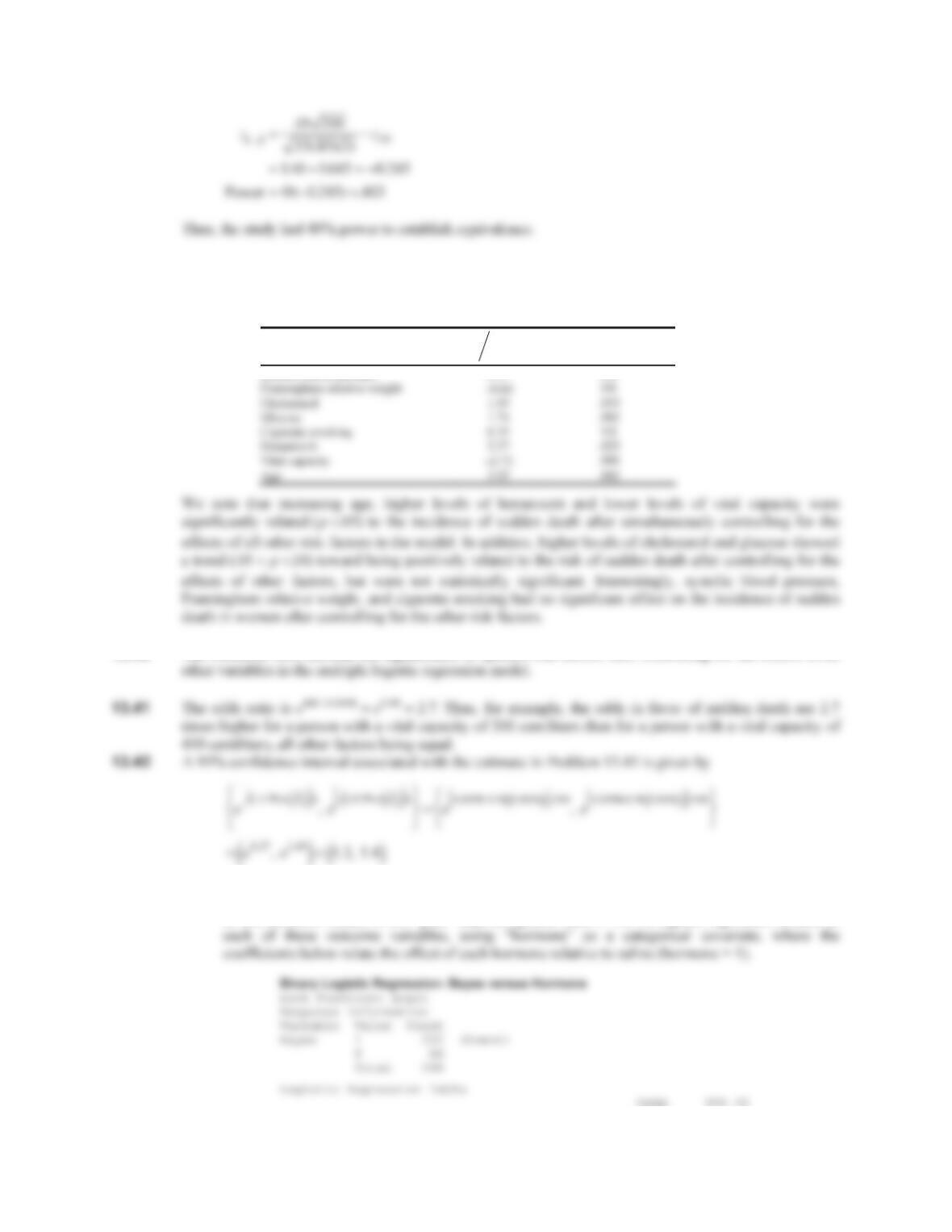
13.38 To estimate the power we refer to Equation 13.48 (in Chapter 13, text), and solve for z1

E

, whereby

CHAPTER 13/DESIGN AND ANALYSIS TECHNIQUES FOR EPIDEMIOLOGIC STUDIES 378

13.39 We compute the ratio of each regression coefficient divided by its standard error. Under the null

hypothesis that a specific risk factor has no effect on sudden death after controlling for all other risk

factors, each such ratio should follow a N(0, 1) distribution. We have the following results

Variable

ˆ

E

ise ˆ

E

i



p-value (2-tailed)

Systolic blood pressure 0.27 NS

13.40 The statistical tests indicate the significance of specific risk factors after controlling for the effects of all

13.43-13.44 For this analysis we create new variables BSyes and PSyes, which serve as indicators of whether

or not secretion values in the “post” state are greater than 0. We fit logistic regression models to

Odds 95% CI