CHAPTER 13/DESIGN AND ANALYSIS TECHNIQUES FOR EPIDEMIOLOGIC STUDIES 379
Predictor Coef SE Coef Z P Ratio Lower Upper
Hormone
2 -1.34571 0.640967 -2.10 0.036 0.26 0.07 0.91
Binary Logistic Regression: Psyes versus Hormone
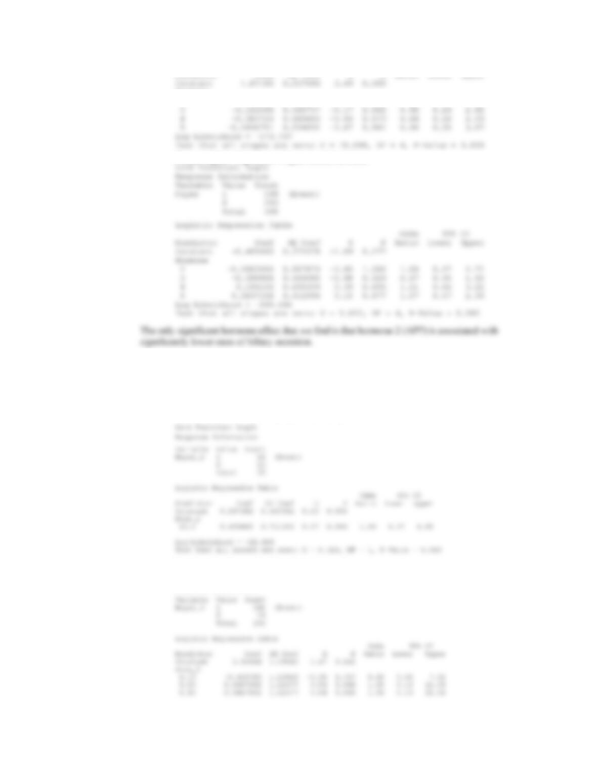
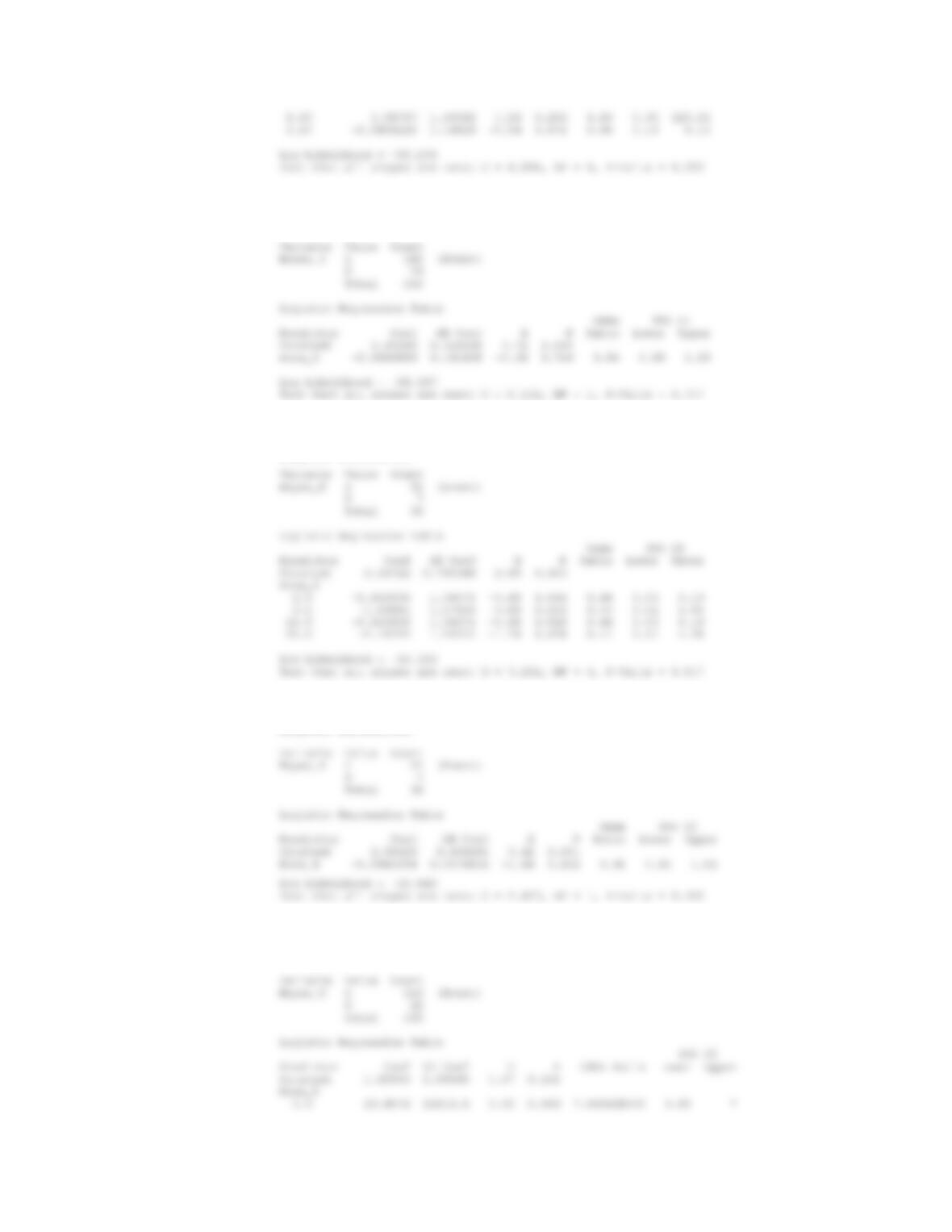
13.45-13.46 Below we show results for both presence of biliary and pancreatic secretions, using dosage levels
as both a linear or categorical predictor. In the case of hormone 2 (APP), we fit only one model,
since there are only dosages of hormone observed. We show results for biliary secretion first, in
which no dose-response effects were observed to be significant at the 0.05 level.
Binary Logistic Regression: Bsyes_2 versus Dose_2
Binary Logistic Regression: Bsyes_3 versus Dose_3
Link Function: Logit
Response Information
CHAPTER 13/DESIGN AND ANALYSIS TECHNIQUES FOR EPIDEMIOLOGIC STUDIES 380
Binary Logistic Regression: Bsyes_3 versus Dose_3
Link Function: Logit
Response Information
Binary Logistic Regression: Bsyes_4 versus Dose_4
Link Function: Logit
Response Information
Binary Logistic Regression: Bsyes_4 versus Dose_4
Link Function: Logit
Response Information
Binary Logistic Regression: Bsyes_5 versus Dose_5
Link Function: Logit
Response Information
CHAPTER 13/DESIGN AND ANALYSIS TECHNIQUES FOR EPIDEMIOLOGIC STUDIES 381
Binary Logistic Regression: Bsyes_5 versus Dose_5
Link Function: Logit
Response Information
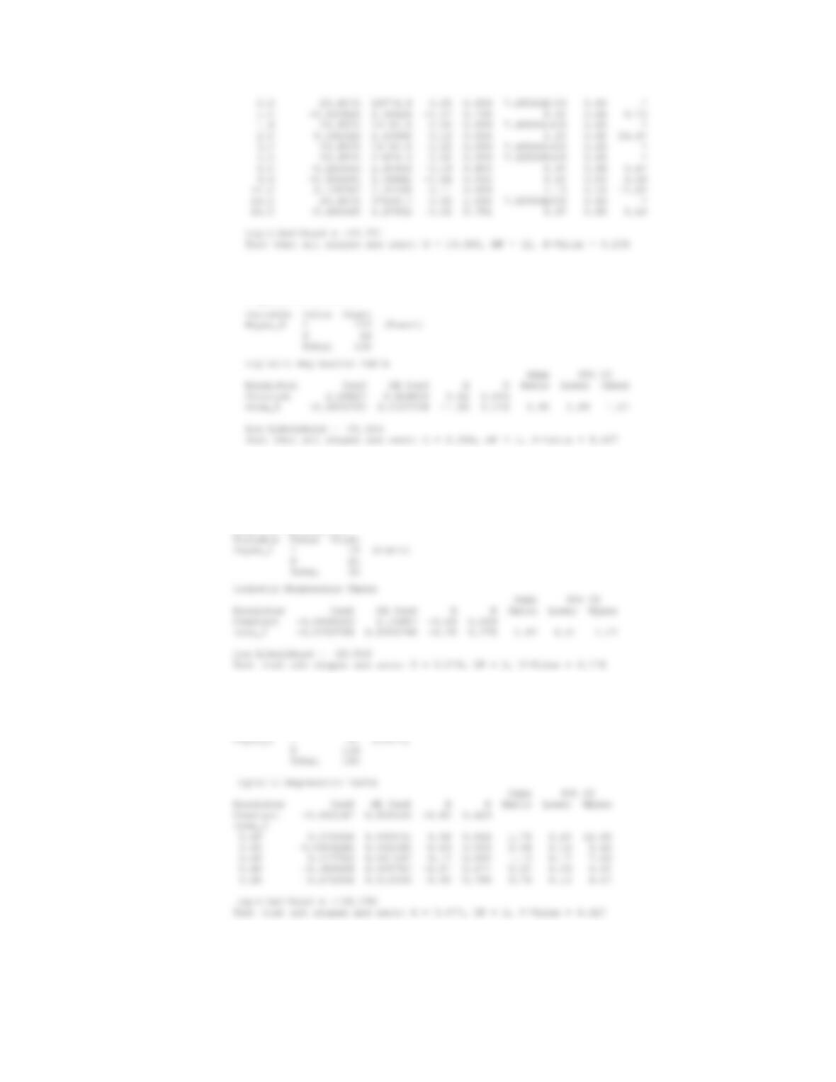
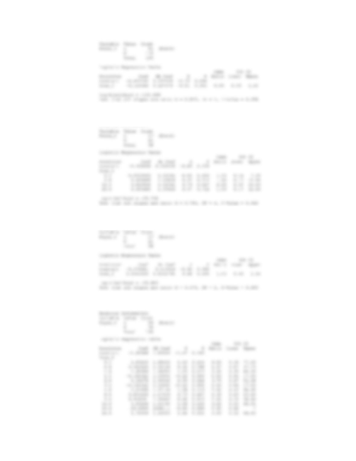
Results for presence of pancreatic secretions are shown below, again with no significant dose-
response relationships detected.
Binary Logistic Regression: Psyes_2 versus Dose_2
Link Function: Logit
Response Information
Binary Logistic Regression: Psyes_3 versus Dose_3
Link Function: Logit
Response Information
Variable Value Count
Binary Logistic Regression: Psyes_3 versus Dose_3
Link Function: Logit
Response Information
CHAPTER 13/DESIGN AND ANALYSIS TECHNIQUES FOR EPIDEMIOLOGIC STUDIES 382
Binary Logistic Regression: Psyes_4 versus Dose_4
Link Function: Logit
Response Information
Binary Logistic Regression: Psyes_4 versus Dose_4
Link Function: Logit
Response Information
Binary Logistic Regression: Psyes_5 versus Dose_5
Link Function: Logit
CHAPTER 13/DESIGN AND ANALYSIS TECHNIQUES FOR EPIDEMIOLOGIC STUDIES 383
Binary Logistic Regression: Psyes_5 versus Dose_5
Link Function: Logit
Response Information
13.47 For this analysis, we use MINITAB’s “store descriptive statistics” option to create our new variables
Totclear and Totears, denoting the sum and number of observations of the variable ‘clear’ for each id.
Then we create the variable cured = (1 if Totclear = Totears, 0 otherwise). We show the logistic
regression output below.
Binary Logistic Regression: cured versus Age_, Antibo_, Totears
Link Function: Logit
Response Information
Variable Value Count
Logistic Regression Table
Odds 95% CI
Predictor Coef SE Coef Z P Ratio Lower Upper
Constant -0.0786038 0.750565 -0.10 0.917
Age_
7
6
Delta Chi-Square versus Probability
9
8
7
Delta Beta (Stand) versus Probability
CHAPTER 13/DESIGN AND ANALYSIS TECHNIQUES FOR EPIDEMIOLOGIC STUDIES 384
goodness-of-fit of the model, we notice that we have what appear to be two outlying observations in both
the “Squared Residuals” and “Delta Beta” plots above. Furthermore, the goodness-of-fit results displayed
in the model output all have rather low p-values suggesting that our overall fit is not ideal.
13.48 For this analysis, we use STATA’s “xtgee” command, with the option family(binomial), which
fits a logistic regression model. We first use the command ‘xtset id’, which identifies the variable ‘id’ as
our clustering variable.
xtset id
xi: xtgee clear antibo i.age, family(binomial)
i.age _Iage_1-3 (naturally coded; _Iage_1 omitted)
——————————————————————————
clear | Coef. Std. Err. z P>|z| [95% Conf. Interval]
13.49-13.51 To calculate our efficacy scores, we use the coding
One-Sample T: Dmax, D12, Dav
Test of mu = 0 vs not = 0
13.52-13.54 For these analyses, we create new variables M = mean(Period 2 score, Period 4 score) for each
patient. Then we perform two-sample t-tests of the values Mmax, M12, and Mav, using treatment
assignment to denote the groups. We find no evidence of carry-over effect for any of the pain scores.
Two-Sample T-Test and CI: Mmax, Drg_ord
CHAPTER 13/DESIGN AND ANALYSIS TECHNIQUES FOR EPIDEMIOLOGIC STUDIES 385
Two-Sample T-Test and CI: M12, Drg_ord
Two-sample T for M12
Two-Sample T-Test and CI: Mav, Drg_ord
Two-sample T for Mav
13.55-13.57 We will first test for treatment effects on both SBP and DBP for each study. Before we can do
this, we first average over the 9 blood pressure observations recorded for each person within each
treatment period, which we denote simply as “Sys” and “Dias”. We then use STATA to reshape the data
——————————————————————————
Variable | Obs Mean Std. Err. Std. Dev. [95% Conf. Interval]
CHAPTER 13/DESIGN AND ANALYSIS TECHNIQUES FOR EPIDEMIOLOGIC STUDIES 386
One-sample t test
——————————————————————————
Variable | Obs Mean Std. Err. Std. Dev. [95% Conf. Interval]
——————————————————————————
Variable | Obs Mean Std. Err. Std. Dev. [95% Conf. Interval]
———+——————————————————————–
——————————————————————————
Variable | Obs Mean Std. Err. Std. Dev. [95% Conf. Interval]
———+——————————————————————–
Next we show tests for carryover effects in each study, for each blood pressure measurement. First, we
CHAPTER 13/DESIGN AND ANALYSIS TECHNIQUES FOR EPIDEMIOLOGIC STUDIES 387
——————————————————————————
Group | Obs Mean Std. Err. Std. Dev. [95% Conf. Interval]
———+——————————————————————–
1 | 6 118.8426 7.111913 17.42056 100.5608 137.1243
——————————————————————————
Group | Obs Mean Std. Err. Std. Dev. [95% Conf. Interval]
———+——————————————————————–
. ttest mean3sys, by(period2)
Two-sample t test with equal variances
——————————————————————————
Group | Obs Mean Std. Err. Std. Dev. [95% Conf. Interval]
. ttest mean1dias, by(period1)
Two-sample t test with equal variances
——————————————————————————
Group | Obs Mean Std. Err. Std. Dev. [95% Conf. Interval]
CHAPTER 13/DESIGN AND ANALYSIS TECHNIQUES FOR EPIDEMIOLOGIC STUDIES 388
———+——————————————————————–
diff | -8.462966 6.508604 -24.38895 7.463014
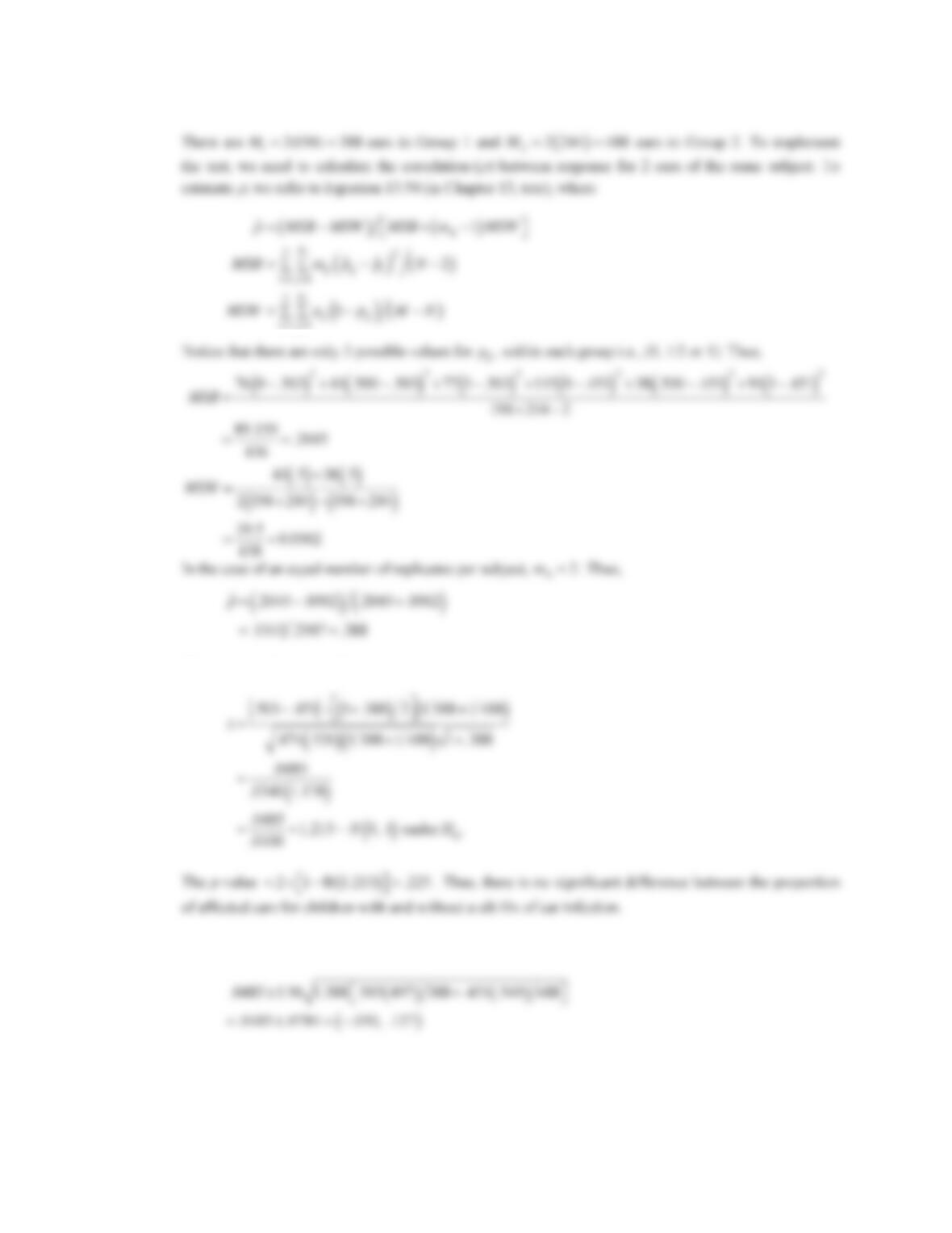
13.58-13.61 The sample sizes required for each of these studies described can be obtained using the same
formula, given in Eq. 13.53,
13.62 We will use a two-sample test for binomial proportions, but will adjust for clustering. Since there are an
CHAPTER 13/DESIGN AND ANALYSIS TECHNIQUES FOR EPIDEMIOLOGIC STUDIES 389
The test statistic is given by
13.63 Referring to Equation 13.47 (in Chapter 13, text), a 95% CI for 12
pp is given by
13.64 In order to use GEE methods in STATA, we need to input data in the following format shown below,
after which we must convert the data set to “panel data” using the xtset command.
CHAPTER 13/DESIGN AND ANALYSIS TECHNIQUES FOR EPIDEMIOLOGIC STUDIES 390
group count leftear inf history
1 76 0 0 1
1 76 1 0 1
2 21 0 1 1
xtset group
We then use the “xtgee” command , which will use an exchangeable correlation structure by default. The
output is shown below.
——————————————————————————
inf | Coef. Std. Err. z P>|z| [95% Conf. Interval]
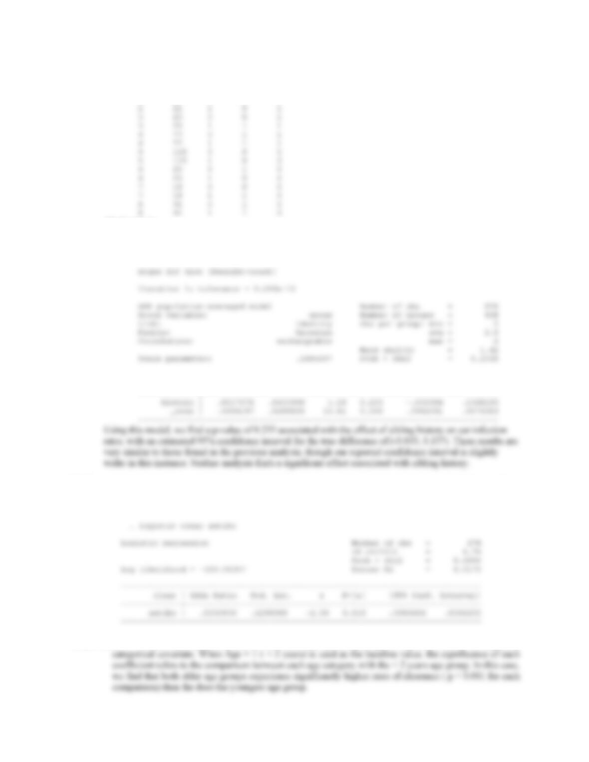
13.65 Using logistic regression techniques in STATA, we can see that variable Antibo (1 = CEF / 2 = AMO) is
significantly related to clearance rate, with a p-value of 0.01 and an estimated odds ratio < 1, suggesting
that AMO is less effective at clearing infection.
13.66-13.67 We can address both questions simultaneously by fitting a logistic regression model with age as a
CHAPTER 13/DESIGN AND ANALYSIS TECHNIQUES FOR EPIDEMIOLOGIC STUDIES 391
——————————————————————————
13.68 The point estimate of RR e
FFQ
0163 085
... A 95% CI for RRFFQ is given by
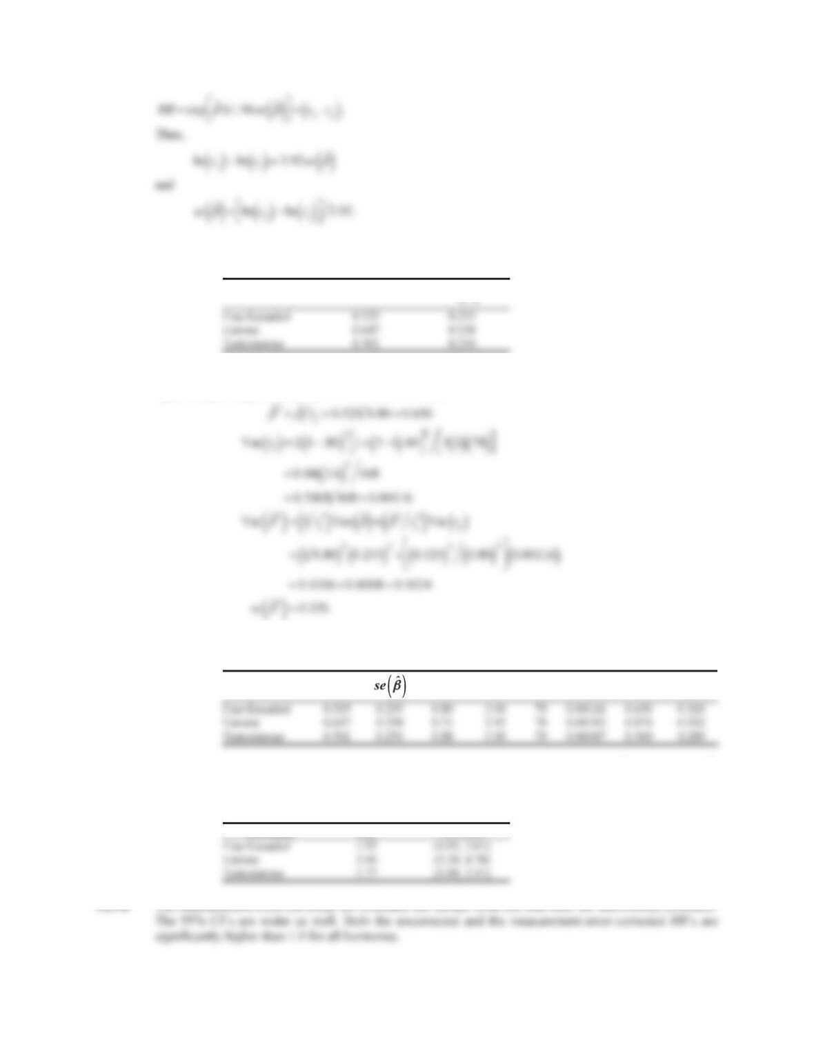
13.70 We refer to Equation 13.73 (in Chapter 13, text). The point estimate of RR
D
R is
13.71 The variance of *
E
is
D
D
CHAPTER 13/DESIGN AND ANALYSIS TECHNIQUES FOR EPIDEMIOLOGIC STUDIES 392
The values for
E
and
se ˆ
E
are given for each hormone in Table 13.51 as follows:
Hormone
E
se ˆ
E
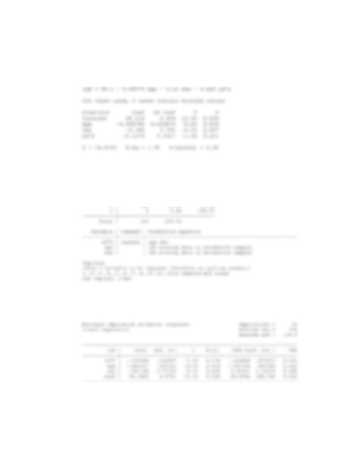
13.74 We refer to Equation 13.73 (in Chapter 13, text). For free estradiol, there were 79 subjects and 3
replicates per subject. Thus, n179 and k03 . Also,
The results for all 3 hormones are given below.
Hormone
E
rI0
k1
n
Var r
I
ˆ
E
ˆ
E
se
13.75 We have the measurement-error-corrected estimated
OR exp ˆ
E
*
. The 95%
CI exp ˆ
E
*
r1.96se ˆ
E
*
ª
¼
¼
.
These are given as follows:
Hormone OR 95% CI
CHAPTER 13/DESIGN AND ANALYSIS TECHNIQUES FOR EPIDEMIOLOGIC STUDIES 393
13.77 In this analysis, we have three incomplete cases due to missing values of 1972 lead level, and we find a
non-significant (p=0.21) negative effect of lead on full-scale IQ.
Regression Analysis: Iqf versus Age, Sex, Ld72
The regression equation is
13.78 We use STATA’s “ice” and “mim” commands to first generate imputed data, and then combine results
over the multiple imputed data sets. Coding is shown. It should be noted that newer versions of STATA
will use different coding (see “mi impute”).
. ice ld72 age sex using imputed, m(10)
#missing |
values | Freq. Percent Cum.
————+———————————–
At this point we have generated 10 new complete data sets, each with different imputed values for our
missing lead observations. The following code will fit a linear regression model to each of the imputed data
sets, and then combine the results in accordance with the guidelines given in the textbook.
. mim: regress iqf ld72 age sex
——————————————————————————
Using this method, we find a negative, but non-significant relationship (p=0.22) between lead levels and
full-scale IQ.
CHAPTER 13/DESIGN AND ANALYSIS TECHNIQUES FOR EPIDEMIOLOGIC STUDIES 394
13.80 We use the chi square test for 22utables.
13.81 34 1500
RR 0.50.
68 1500
13.82 We use the Mantel-Haenszel test. We have the test statistic:
24.64 55.62 80.26
Thus, the test statistic is
CHAPTER 13/DESIGN AND ANALYSIS TECHNIQUES FOR EPIDEMIOLOGIC STUDIES 395
13.83 In the total population there are 3000 women without preexisting fractures and 1500 women with
preexisting fractures. Thus, the standardized risk ratio is
13.86 ( | ) 18 / 200 4.5
( | ) 10 / 500
P hypertensive obese
RR P hypertensive normal
CHAPTER 13/DESIGN AND ANALYSIS TECHNIQUES FOR EPIDEMIOLOGIC STUDIES 396
13.88 The estimated OR for hypertension comparing Hispanic boys vs. Caucasian boys is
13.94 We will use the Mantel-Haenszel test. We construct 2 u 2 tables relating MI and severe vertex baldness
for each age group
60 MI >60 MI
yes no yes no