CHAPTER 12/MULTISAMPLE INFERENCE 341
To perform our repeated regression analyses and store the parameters, we need to use the following code,
which stores the estimated intercept for person in variable B1, and the slope in variable B2. Depending on
how the data was initially entered, we need to check to make sure that our variable representing NAPAP
group has not been “unstacked”.
summarize(id)
egen ID = group(id)
For each person, the estimated intercept (B1) represents the fitted baseline serum-creatinine value observed
anova B1 napap
Source | Partial SS df MS F Prob > F
| Summary of B2
NAPAP | Mean Std. Dev. Freq.
Analysis of Variance
Source SS df MS F Prob > F
CHAPTER 12/MULTISAMPLE INFERENCE 342
Row Mean-|
Col Mean | 1 2
12.52 When we fit a one-way random effect ANOVA to data, we obtain the following.
General Linear Model: Base versus ID
Factor Type Levels Values
Analysis of Variance for Base, using Adjusted SS for Tests
Source DF Seq SS Adj SS Adj MS F P
Our estimate of intraclass correlation is given by 222
ˆˆˆˆ
/( )
AA
U
VVV
Where
2
ˆ()/
A between within
M
SMSn
V
12.53-12.54
For this analysis, we will use the change values calculated in 12.21-12.26, in order to eliminate some
variability, as subjects had vastly different baseline readings. Within each preparation group, we want
CHAPTER 12/MULTISAMPLE INFERENCE 343
change | Coef. Std. Err. t P>|t| [95% Conf. Interval]
. reg change weeks if prepar==2
Source | SS df MS Number of obs = 24
Source | SS df MS Number of obs = 20
————-+—————————— F( 1, 18) = 1.24
——————————————————————————
. reg change weeks if prepar==4
Source | SS df MS Number of obs = 24
12.55 We use the same random-effects ANOVA models that were fit in 12.35, which are shown below.
General Linear Model: Estrone versus Subject
CHAPTER 12/MULTISAMPLE INFERENCE 344
Our estimate of intraclass correlation is given by
ˆ
U
ˆ
V
A
2
/(ˆ
V
A
2
ˆ
V
2
)
Where
The confidence interval (c1, c2) is given by,
General Linear Model: Androste versus Subject
Factor Type Levels Values
Our estimate of intraclass correlation is given by 222
ˆˆˆˆ
/( )
AA
U
VVV
Where
The confidence interval (c1, c2) is given by
General Linear Model: Testost versus Subject
CHAPTER 12/MULTISAMPLE INFERENCE 345
Our estimate of intraclass correlation is given by 222
ˆˆˆˆ
/( )
AA
U
VVV
Where
The confidence interval (c1, c2) is given by,
12.57 We test the hypotheses:
1
i
12.58 Our best estimate of the within-group variance is given by:
12.59 We have the test statistic:
CHAPTER 12/MULTISAMPLE INFERENCE 346
12.60 Referring to Table 8, text, we see that
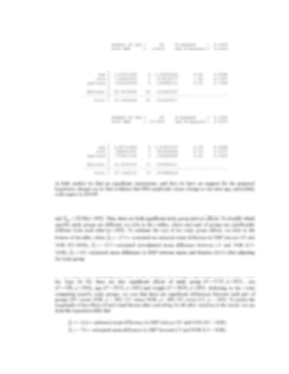
12.61 There are many ways to interpret and answer this question, but it seems we are interested only in the
0.02 .04 .06 .08
Density
010 20 30
A_amp
0.001 .002 .003 .004 .005
Density
0500 1000 1500
B_amp
CHAPTER 12/MULTISAMPLE INFERENCE 347
. anova lnbamp age cond age*cond if group==1
Source | Partial SS df MS F Prob > F
———–+—————————————————-
Model | 4.39733932 8 .549667415 1.76 0.0973
. anova lnaamp age cond age*cond if group==1
Source | Partial SS df MS F Prob > F
———–+—————————————————-
Model | 4.54125989 8 .567657486 1.24 0.2916
12.62 The overall F statistic is 13415 001..p
indicating that at least some of the variables in the model have
non-zero regression coefficients. Referring to the Type III SS, we see that Fp
study group
194 49 001..
12.63 The results are similar to those of Problem 12.58. There are significant overall effects,
CHAPTER 12/MULTISAMPLE INFERENCE 348
12.64 We use the F test for one-way ANOVA. The test statistic is F = Between MS / Within MS 1,knk
F
under H0. In this case,
12.65 We perform the t test for each pair of groups. We will label the groups as A = placebo, B = simivastatin
plus niacin, C = antioxidants, and D = simivastatin plus niacin plus antioxidants. The results are as
follows:
Groups t-statistic p-value*
A vs. B
0.4 3.9 15.58 1 34 1 33 4.46 <.001
CHAPTER 12/MULTISAMPLE INFERENCE 349
12.66 The linear contrast 4231
0.7 0.4 1.8 3.9 3.2Ly y y y . Its standard error is given by
12.67 For each of the analyses in 12.63–12.67, we use the ln–transformation of the TBUT scores, as described
reshape long imchange, i(id) j(sec)
anova imchange id sec
Source | Partial SS df MS F Prob > F
———–+—————————————————-
Model | 8.94539613 15 .596359742 2.65 0.0143
12.68 We repeat the same analysis as in 12.63, but with the 5 minute post-installation data. Again, we find
significant differences by person, but not by non-blink time.
Data wide -> long
——————————————————————–
CHAPTER 12/MULTISAMPLE INFERENCE 350
12.69 At 10 minutes post-installation, we find no significant differences.
Source | Partial SS df MS F Prob > F
12.70 At 15 minutes post-installation, we still see no significant differences.
Source | Partial SS df MS F Prob > F
———–+—————————————————-
Model | 8.97608916 15 .598405944 1.59 0.1448
12.72 Since there are 10 comparisons, we require a nominal .05 10 .005
D
to achieve statistical significance
12.73 We first reorder the SNP’s by size of the nominal p-value as shown below:
i SNP
nominal
p-value (pi) qi FDR
i
1 7 .001 .010 .010
CHAPTER 12/MULTISAMPLE INFERENCE 351
12.74 A reasonable model would be a one-way random-effects model using a ln-transformation,
12.75 To fit this model, we can enter the following into MINITAB, and then use the “General Linear Model”
command to fit our random-effects ANOVA model.
ID lnTBUT
1 1.57
1 1.87
General Linear Model: lnTBUT versus ID
Analysis of Variance for lnTBUT, using Adjusted SS for Tests
CHAPTER 12/MULTISAMPLE INFERENCE 352
Where
2
ˆ()/
A between within
MS MS n
V
12.79 In this case, our F statistic = Between MS / Within MS = 0.0122/0.0038 = 3.21 ~ F(3,2850) under the
12.80 (i) Using the LSD method, we can use the MINITAB two-sample t-test command using summary
Two-Sample T-Test and CI
Sample N Mean StDev SE Mean
1 267 0.4350 0.0616 0.0038
12.81 In this case, we could use a linear regression model, with BMD as the outcome and Score as the
12.83 The test statistic is F = Between MS / Within MS 1,knk
F
under H0. In this case,
CHAPTER 12/MULTISAMPLE INFERENCE 353
12.84 For the Bonferroni comparisons, we will use the pooled estimate s = sqrt(Within MS) = 1.29. Any pair with
a t-statistic > 2.68 will be considered significantly different at the 0.05 level. Comparisons are shown
below.
Groups t-statistic Significant?
A vs. B
72.73 66.26 1.66 1/ 22 1 43 19.16
Y
12.85 We would use a two-way ANOVA model of the form
ijk i j ij ijk
y
P
D
EJ
H
, where
Represents the wing length of the kth bird in the ith gender of the jth subspecies
12.86 In total, we have 10 different outcome variables (5 measurements, evaluated at 14 days and 7 days relative
to baseline. First we create these 10 difference variables, where “_diff1” refers to day 7 – day 0, and
y
CHAPTER 12/MULTISAMPLE INFERENCE 354
General Linear Model: cdiff1, sdiff1, … versus tr
Factor Type Levels Values
tr fixed 3 1, 2, 3
Analysis of Variance for cdiff1, using Adjusted SS for Tests
Source DF Seq SS Adj SS Adj MS F P
Analysis of Variance for idiff1, using Adjusted SS for Tests
Source DF Seq SS Adj SS Adj MS F P
Analysis of Variance for tdiff1, using Adjusted SS for Tests
Source DF Seq SS Adj SS Adj MS F P
Analysis of Variance for ndiff1, using Adjusted SS for Tests
Source DF Seq SS Adj SS Adj MS F P
Analysis of Variance for cdiff2, using Adjusted SS for Tests
Source DF Seq SS Adj SS Adj MS F P
Analysis of Variance for sdiff2, using Adjusted SS for Tests
Source DF Seq SS Adj SS Adj MS F P
CHAPTER 12/MULTISAMPLE INFERENCE 355
Analysis of Variance for tdiff2, using Adjusted SS for Tests
Source DF Seq SS Adj SS Adj MS F P
Below, we show confidence intervals for the effect of each drug (treatment = 1, 2) relative to placebo
(treatment = 3), using the Bonferroni method for multiple comparisons. Mildly significant treatment effects
are highlighted below, both of which refer to treatment 2 (drug G)
Bonferroni 95.0% Simultaneous Confidence Intervals
Response Variable sdiff1
Comparisons with Control Level
tr = 3 subtracted from:
tr Lower Center Upper +———+———+———+——
Bonferroni Simultaneous Tests
Response Variable sdiff1
Comparisons with Control Level
tr = 3 subtracted from:
Bonferroni 95.0% Simultaneous Confidence Intervals
Response Variable tdiff1
Comparisons with Control Level
tr = 3 subtracted from:
tr Lower Center Upper —+———+———+———+—
Bonferroni Simultaneous Tests
Response Variable tdiff1
Comparisons with Control Level
tr = 3 subtracted from:
Difference SE of Adjusted
Bonferroni 95.0% Simultaneous Confidence Intervals
Response Variable sdiff2
CHAPTER 12/MULTISAMPLE INFERENCE 356
-1.5 0.0 1.5 3.0
Bonferroni Simultaneous Tests
12.87 In order to address this question, we first recode our difference variables so that each time period has five
First1 First2 First3 First4 First5 Second1 Second2 Second3 Second4 Second5
5 0 0 0 0 5 5 -10 0 0
reshape long first, i(obs) j(loc)
anova first tr loc
Source | Partial SS df MS F Prob > F
CHAPTER 12/MULTISAMPLE INFERENCE 357
Source | Partial SS df MS F Prob > F
———–+—————————————————-
Model | 301.056277 14 21.5040198 1.68 0.0553
. anova second tr loc
Number of obs = 910 R-squared = 0.0126
Root MSE = 3.45134 Adj R-squared = 0.0061
Source | Partial SS df MS F Prob > F
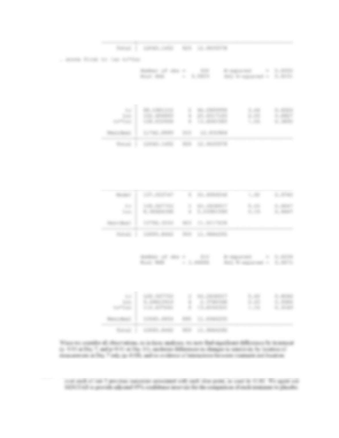
. anova second tr loc tr*loc
Source | Partial SS df MS F Prob > F
———–+—————————————————-
Model | 248.160789 14 17.7257707 1.49 0.1079
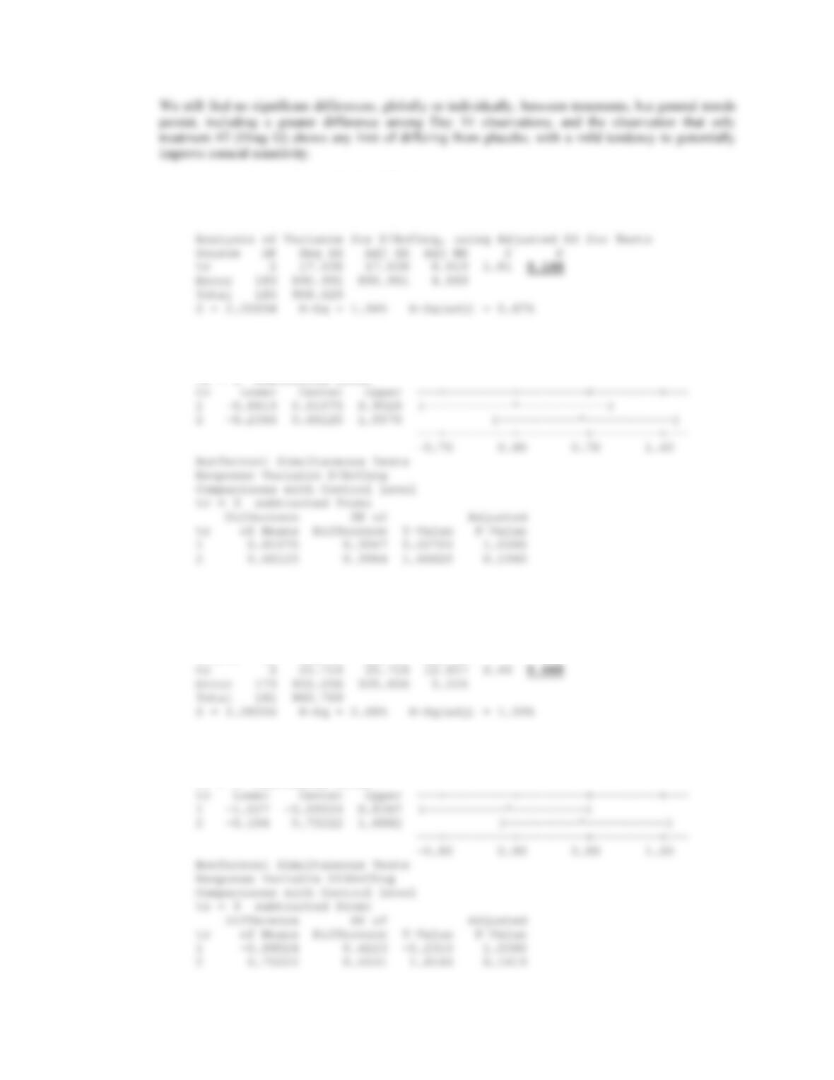
12.88 For this final analysis we create two new outcome variables, Day7AvChng and Day14AvChng, averaging
CHAPTER 12/MULTISAMPLE INFERENCE 358
General Linear Model: D7AvChng versus tr
Factor Type Levels Values
tr fixed 3 1, 2, 3
Bonferroni 95.0% Simultaneous Confidence Intervals
Response Variable D7AvChng
Comparisons with Control Level
tr = 3 subtracted from:
General Linear Model: D14AvChng versus tr
Factor Type Levels Values
tr fixed 3 1, 2, 3
Analysis of Variance for D14AvChng, using Adjusted SS for Tests
Source DF Seq SS Adj SS Adj MS F P
Bonferroni 95.0% Simultaneous Confidence Intervals
Response Variable D14AvChng
Comparisons with Control Level
tr = 3 subtracted from: