323
MULTISAMPLE
INFERENCE
12.1 We can use the one–way analysis of variance to test the hypothesis
H
H
01 2 3 1
::
P
P
P
versus at least
12.3 We use the test statistic
t y
1
y
2
s
2
1
n
1
1
n
2
§
©
¨
¨
·
¹
¸
¸
~t
nk
under
H
0.The results are given for each pair of groups as
M
H
H
CHAPTER 12/MULTISAMPLE INFERENCE 324
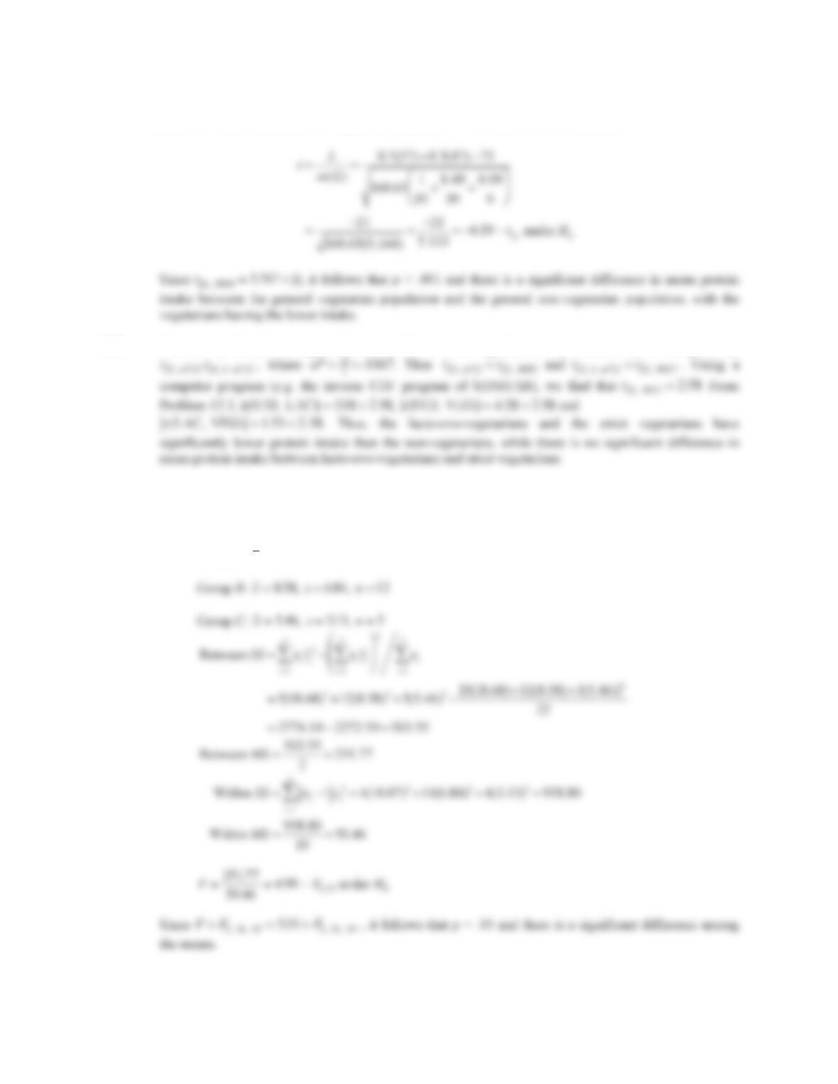
12.4 This contrast is an estimate of the difference in mean protein intake between the general vegetarian
population and the general non-vegetarian population. We compute the test statistic:
12.5 We use the Bonferroni approach. For a 5% level of significance, the critical values are given by
12.6 We wish to test the hypothesis
H
H
i01
0: all versus
D
: at least one
D
iz0. We will use the fixed effects
one–way ANOVA. For this purpose, we compute the mean and standard deviation for each group as
follows:
Group A:
x
s
n 18 68 10 07 5., .,
x
s
x
s
CHAPTER 12/MULTISAMPLE INFERENCE 325
12.7 We use the test statistic:
t y
1
y
2
s
2
1
n
1
1
n
2
§
©
¨
¨
·
¹
¸
¸
~t
nk
under H
0
.
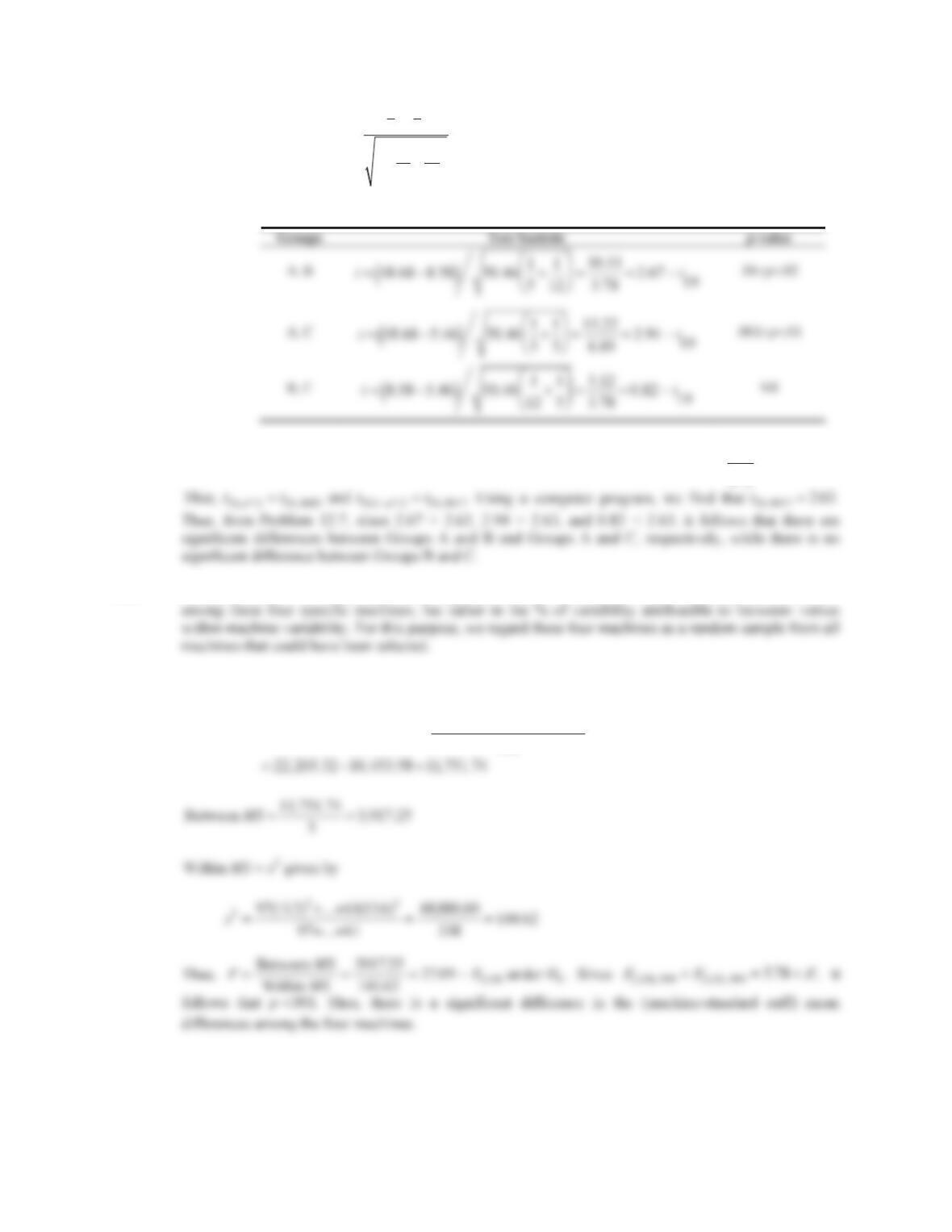
The results are given for each pair of groups
as follows:
12.8 Under the Bonferroni method, the critical values are given
t
19,
D
*/2
,t
19,1
D
*/2
, where
D
* .05
C
.0167.
12.9 A random effects one-way ANOVA is appropriate here because we are not interested in differences
12.10 We perform the overall F test for one-way ANOVA as follows:
Between SS 98(0.5)
2
W62(6.9)
2
[98(0.5)
2
W62(6.9)]
2
342
12.11 The estimated within machine variability
..
V
e
2144 62 The between-machine variability
V
A
2
is
estimated by
CHAPTER 12/MULTISAMPLE INFERENCE 326
12.12 The fixed effects one-way ANOVA.
12.13 The test statistic is F
M
S
M
SFH
knk
Between
Within under ~,10
We have:
M
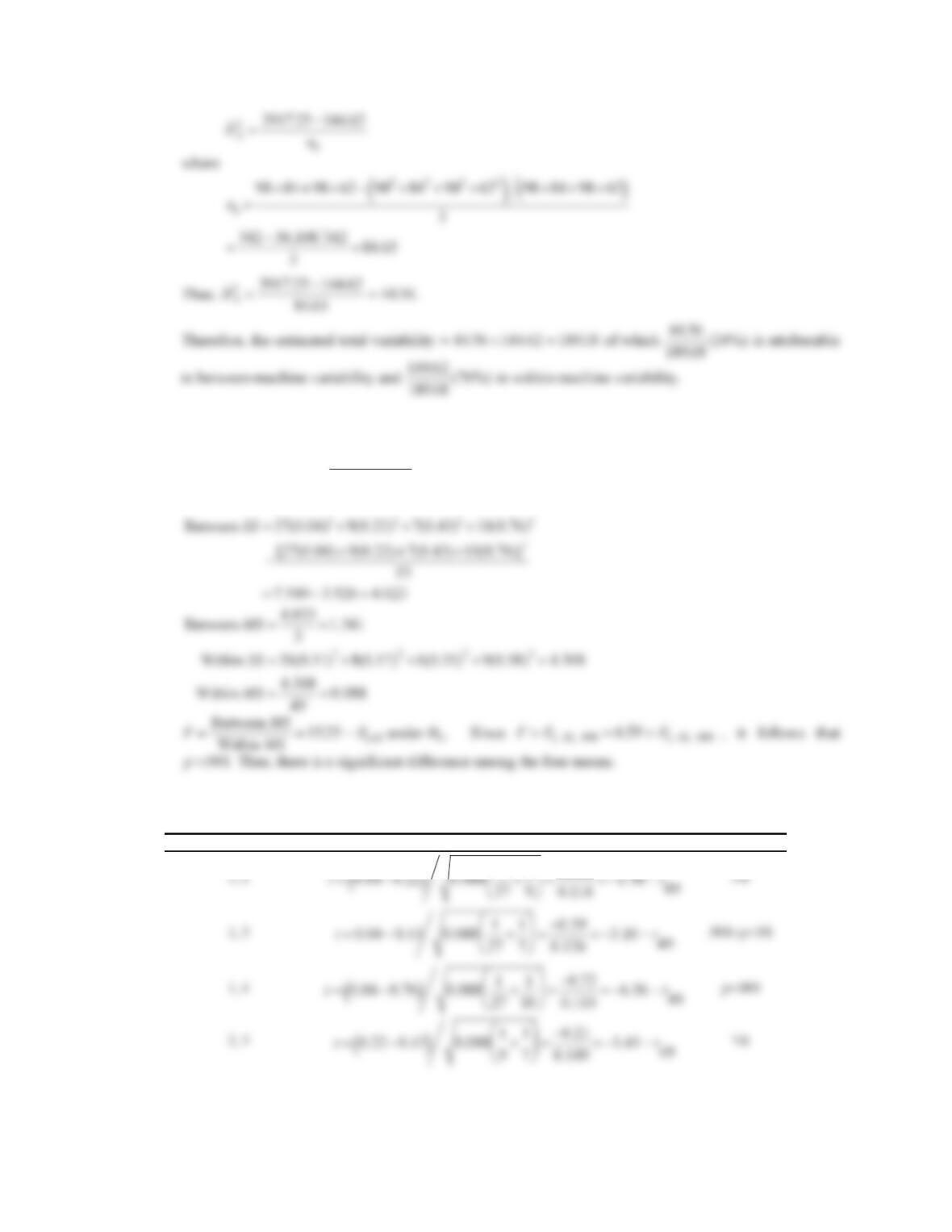
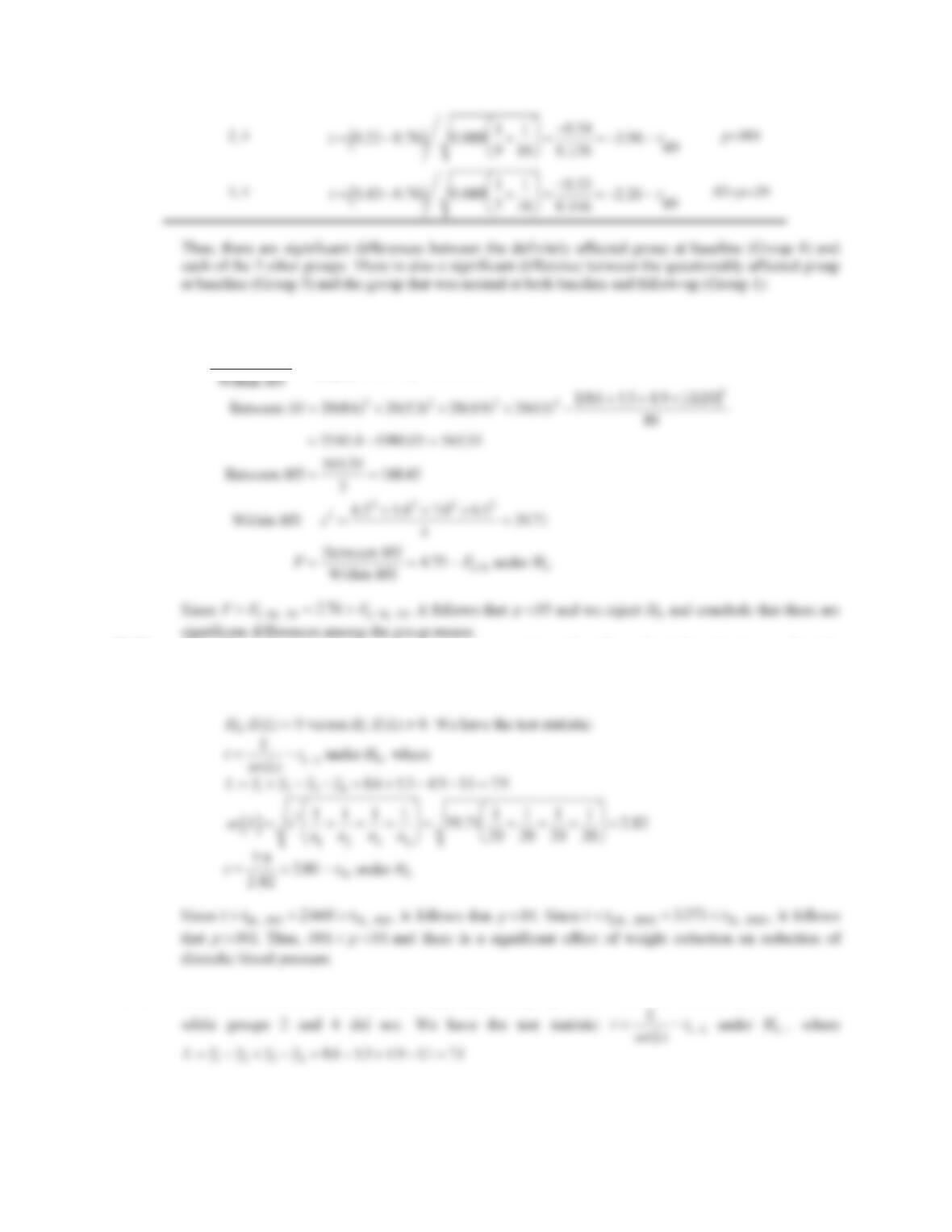
To identify differences between specific groups, we use the LSD procedure, which is summarized as
follows:
Comparison Groups Test Statistic p-value
§
CHAPTER 12/MULTISAMPLE INFERENCE 327
12.14 We will use a fixed effects one-way ANOVA to test the hypothesis
H
H
01 2 3 4 1
::
P
P
P
P
versus at
least two of the
P
i‘s are different. We use the test statistic.
F
M
S
H
knk
Between
,10
We have:
12.15 We will use the contrast
P
P
P
P
P
L
1234
to estimate the effect of weight reduction on diastolic
blood pressure change since groups 1 and 2 received counseling for weight reduction, while groups 3 and
4 did not. We will test the hypothesis
H
H
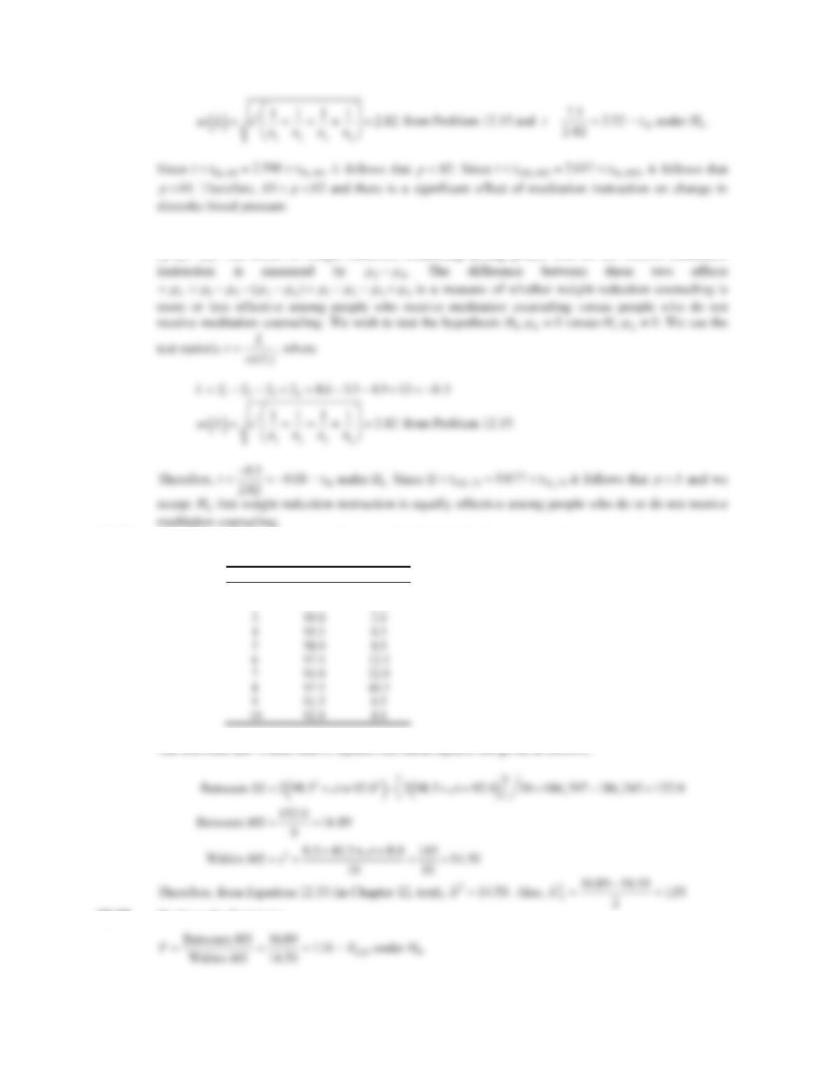
12.16 We will use the contrast
P
P
P
P
P
L
1234
since groups 1 and 3 received counseling for meditation,
H
CHAPTER 12/MULTISAMPLE INFERENCE 328
12.17 The effect of weight reduction counseling among people who receive meditation instruction is measured
by
P
P
. The effect of weight reduction counseling among people who do not receive meditation
12.18 We will use a one-way random effects model ANOVA. We first compute the mean and variance for each
day as follows:
Day Mean Variance
1 98.5 0.5
2 97.5 40.5
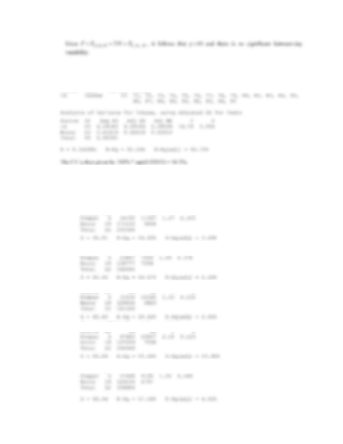
The Between and Within sum of squares and mean squares are given as follows:
12.19 We have the F statistic:
CHAPTER 12/MULTISAMPLE INFERENCE 329
12.20 To answer this question, we use the procedure described in Eq. 12.34. We can use MINITAB’s ANOVA
Æ General Linear Model command, using the ln(baseline values). The output is shown below.
General Linear Model: lnbase versus id
Factor Type Levels Values
12.21-12.25
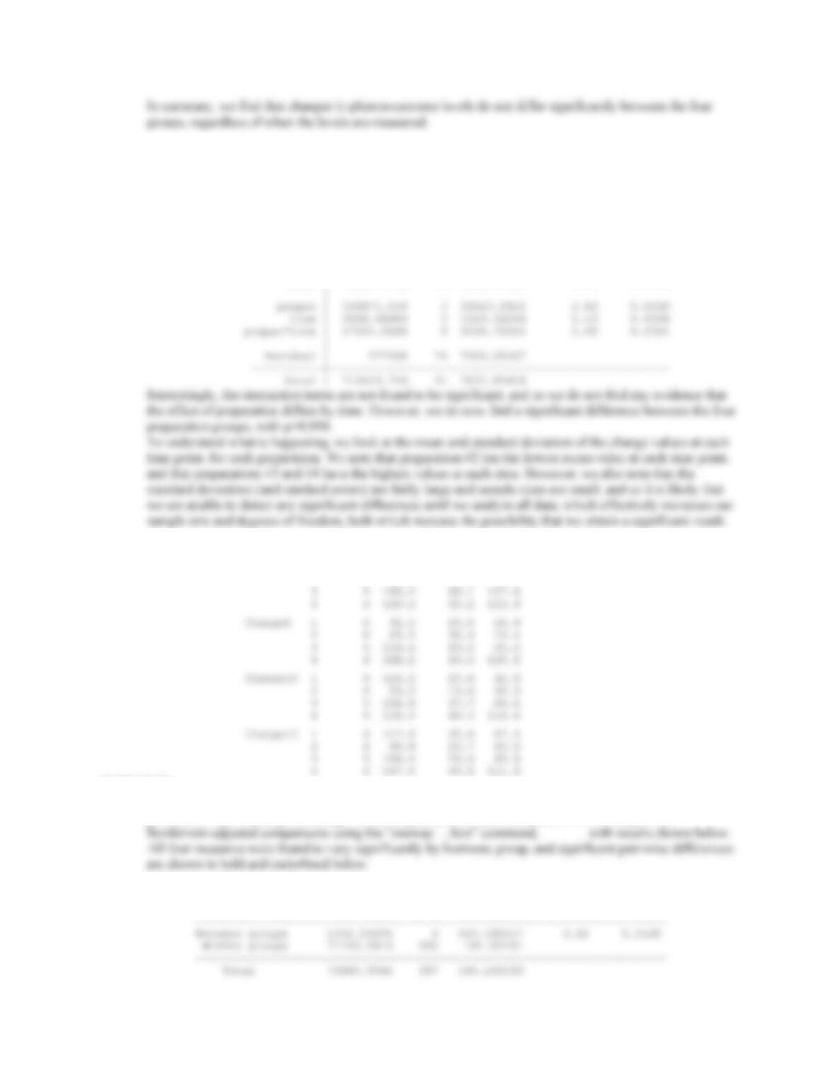
We first need to create our response variables: (Change6, Change8, Change10, Change12, ChangeAv),
which are given by [Week X level – average(baseline 1, baseline 2)]. We then perform one-way ANOVA
to compare mean change values among the 4 preparation groups. Results are shown below.
One-way ANOVA: Change6 versus Prepar
Source DF SS MS F P
One-way ANOVA: Change8 versus Prepar
Source DF SS MS F P
One-way ANOVA: Change10 versus Prepar
One-way ANOVA: Change12 versus Prepar
One-way ANOVA: ChangeAv versus Prepar
Source DF SS MS F P
CHAPTER 12/MULTISAMPLE INFERENCE 330
12.26 For this question, we use STATA to perform two-way ANOVA, where our outcome variable is “change
from baseline”, and our factors are preparation and follow-up time.
anova change prepar time prepar*time
Number of obs = 92 R-squared = 0.1945
Root MSE = 87.1395 Adj R-squared = 0.0355
Source | Partial SS df MS F Prob > F
———–+—————————————————-
Model | 139339.739 15 9289.31594 1.22 0.2737
Descriptive Statistics: Change6, Change8, Change10, Change12
Variable Prepar N Mean SE Mean StDev
Change6 1 6 85.5 31.9 78.2
2 6 82.8 25.1 61.4
12.27-12.30
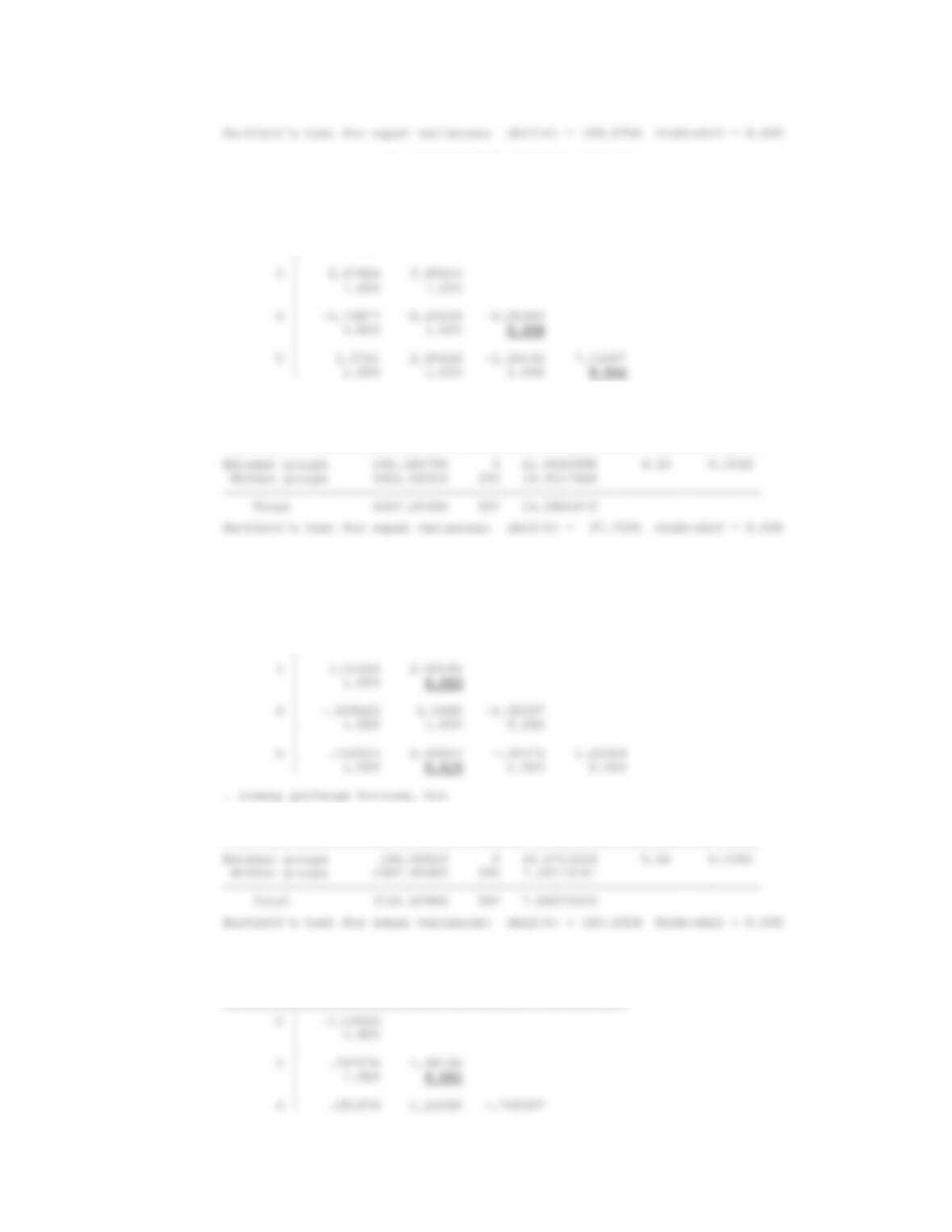
Since we interested in finding any and all significant group differences, we need to use a multiple-testing
procedure. After creating our change variables (post-pre) for each measure, STATA can perform
. oneway bschange hormone, bon
Analysis of Variance
Source SS df MS F Prob > F
CHAPTER 12/MULTISAMPLE INFERENCE 331
Comparison of Bschange by Hormone
(Bonferroni)
Row Mean-|
Col Mean | 1 2 3 4
———+——————————————–
2 | -1.48238
| 1.000
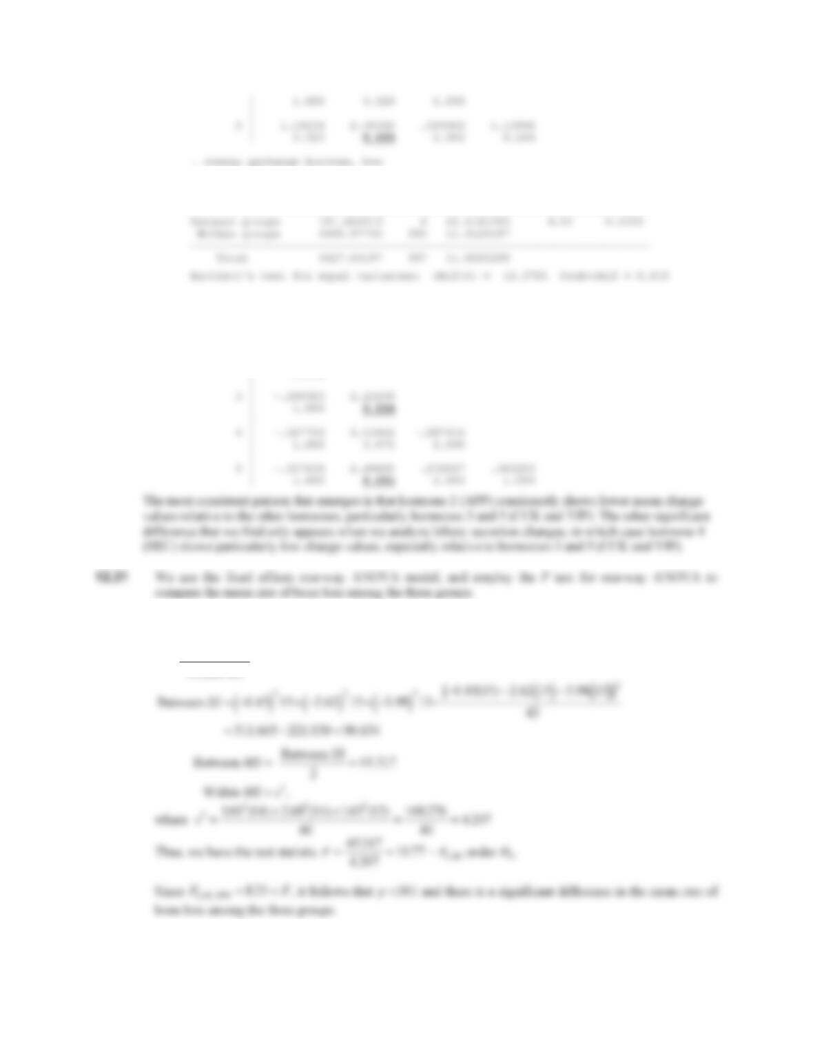
. oneway bpchange hormone, bon
Analysis of Variance
Source SS df MS F Prob > F
Comparison of Bpchange by Hormone
(Bonferroni)
Row Mean-|
Col Mean | 1 2 3 4
———+——————————————–
2 | -1.57762
| 1.000
Analysis of Variance
Source SS df MS F Prob > F
Comparison of Pschange by Hormone
(Bonferroni)
Row Mean-|
Col Mean | 1 2 3 4
CHAPTER 12/MULTISAMPLE INFERENCE 332
Analysis of Variance
Source SS df MS F Prob > F
————————————————————————
Comparison of Ppchange by Hormone
(Bonferroni)
Row Mean-|
Col Mean | 1 2 3 4
———+——————————————–
2 | -2.50238
| 0.030
12.32 We have the test statistic
F
M
S
M
SFH
knk
Between
Within under ~,10
, where
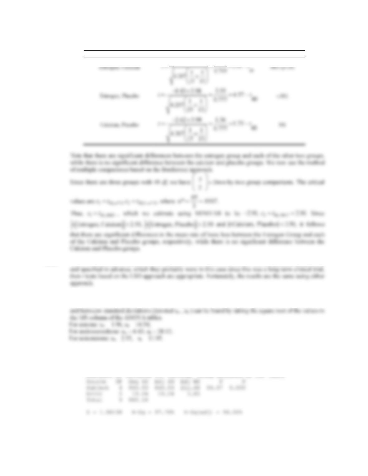
12.33 We first use t tests with critical values based on the LSD procedure as follows
CHAPTER 12/MULTISAMPLE INFERENCE 333
Groups Compared Test Statistic p-value
12.34 There is not a definite answer to this question. In the author’s opinion, if the comparisons are planned
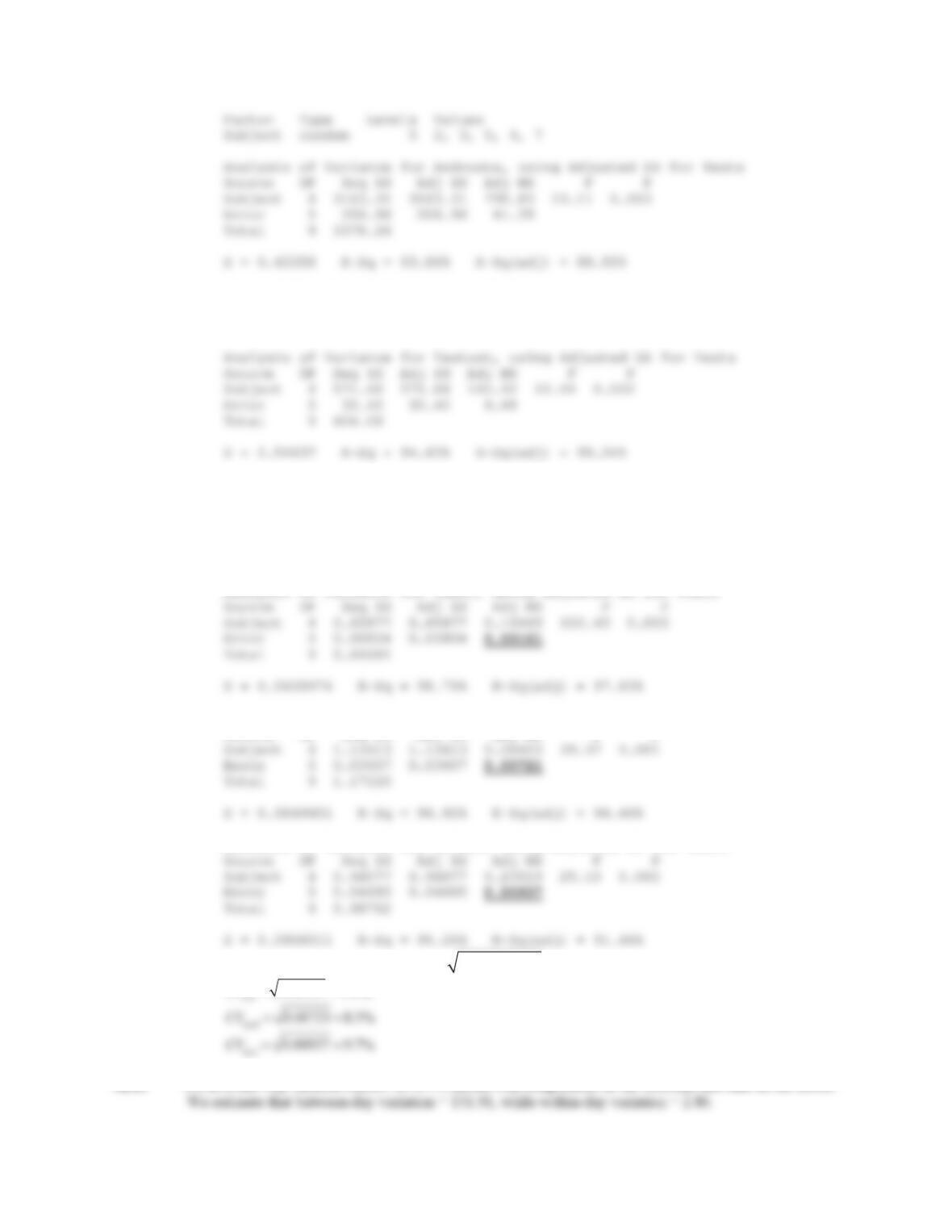
12.35 We use MINITAB’s General Linear Model command to fit a one-way random effect ANOVA, and find
that in each case, within-subject variation is much smaller than between-subject variation. The within-
General Linear Model: Estrone versus Subject
Factor Type Levels Values
Subject random 5 2, 3, 5, 6, 7
General Linear Model: Androste versus Subject
CHAPTER 12/MULTISAMPLE INFERENCE 334
General Linear Model: Testost versus Subject
Factor Type Levels Values
Subject random 5 2, 3, 5, 6, 7
12.36 We use the procedure described in Eq. 12.34 and convert all values to the ln scale before running a one-
way random effects ANOVA.
General Linear Model: lnEst, lnAnd, lnTest versus Subject
Factor Type Levels Values
Subject random 5 2, 3, 5, 6, 7
Analysis of Variance for lnEst, using Adjusted SS for Tests
Analysis of Variance for lnAnd, using Adjusted SS for Tests
Source DF Seq SS Adj SS Adj MS F P
Analysis of Variance for lnTest, using Adjusted SS for Tests
Now, for each hormone, we have that
CV whithin MS
, so we get
CV
0.00161 4.0%
12.37 We fit a one-way random-effects ANOVA model with temperature as the outcome and date as the factor.
CHAPTER 12/MULTISAMPLE INFERENCE 335
Analysis of Variance for In_temp, using Adjusted SS for Tests
Source DF Seq SS Adj SS Adj MS F P
12.38 When we continue to assume a one-way random effects model, with “room” as the factor, we find a
highly significant variation in temperature between different rooms in the house, with p<0.001
General Linear Model: In_temp versus Room
Factor Type Levels Values
12.39 We use the Bonferroni multiple testing option in STATA to address this question. First we show a table
Descriptive Statistics: In_temp
Variable Room Mean
In_temp 1 65.600
2 64.517
Analysis of Variance
Source SS df MS F Prob > F
————————————————————————
CHAPTER 12/MULTISAMPLE INFERENCE 336
Row Mean-|
Col Mean | 1 2 3 4 5 6
———+——————————————————————
2 | -1.08333
| 1.000
|
3 | 1.78333 2.86667
| 1.000 0.019
|
14 | 2.16667 3.25 .383333 .983333 -.05 .783333
| 0.629 0.002 1.000 1.000 1.000 1.000
|
Row Mean-|
Col Mean | 7 8 9 10 11 12
———+——————————————————————
8 | -.316667
| 1.000
CHAPTER 12/MULTISAMPLE INFERENCE 337
|
16 | -1.45 -1.13333 -.716667 -1.1 1.63333 -1.46667
| 1.000 1.000 1.000 1.000 1.000 1.000
|
12.40 Using one-way fixed-effect ANOVA, with “iqf” as the response and “lead_type” as the factor, we find
no evidence for differences in full-scale IQ between exposure groups, with a p-value of 0.24.
. oneway iqf lead_type, bon tabulate
| Summary of Iqf
Lead_type | Mean Std. Dev. Freq.
Analysis of Variance
Source SS df MS F Prob > F
Row Mean-|
Col Mean | 1 2
———+———————-
2 | -3.80405
CHAPTER 12/MULTISAMPLE INFERENCE 338
12.41 We can use MINITAB’s Tukey approach to estimate confidence intervals for multiple comparisons.
These are shown below. We note that “type 1” refers to unexposed, “type 2” refers to currently exposed,
and “type 3” refers to previously exposed.
12.43 We first combine the three samples together and assign ranks to the observations in the combined
sample. Since the individual samples are already ordered, we can do this directly from the data as listed.
We have
Trypsin Secretion
d 50 51-1000 ! 1000
Subject Value Rank Subject Value Rank Subject Value Rank
1 1.7 2.0 1 1.4 1.0 1 2.9 8.0
We then compute the rank sum for each sample. The Kruskal-Wallis test statistic is given by
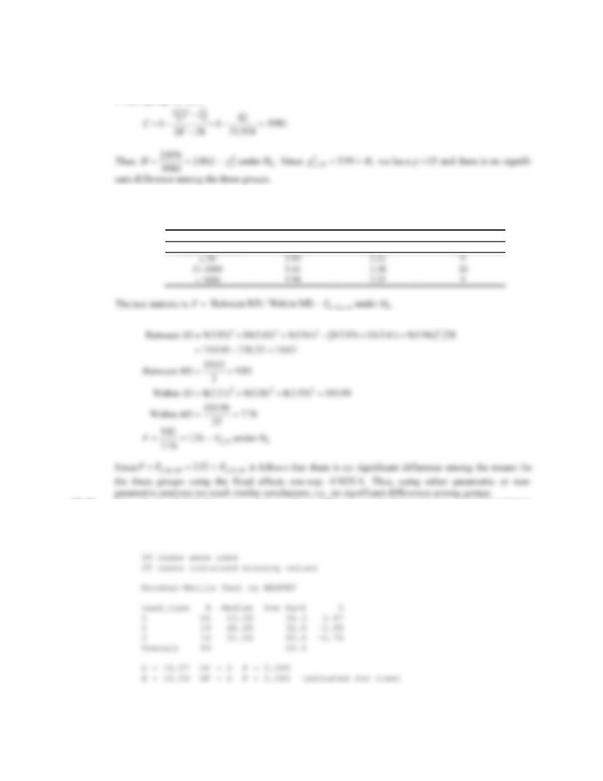
CHAPTER 12/MULTISAMPLE INFERENCE 339
The value C represents the correction factor for ties. Since there are 7 groups of tied values with 2 values
in each group we have
A comparable parametric analysis would be given by the fixed effects one-way ANOVA. We have the
following descriptive statistics for each of the three groups
Mean protein concentration by trypsin secretion group
Trypsin Secretion mean sd n
We have
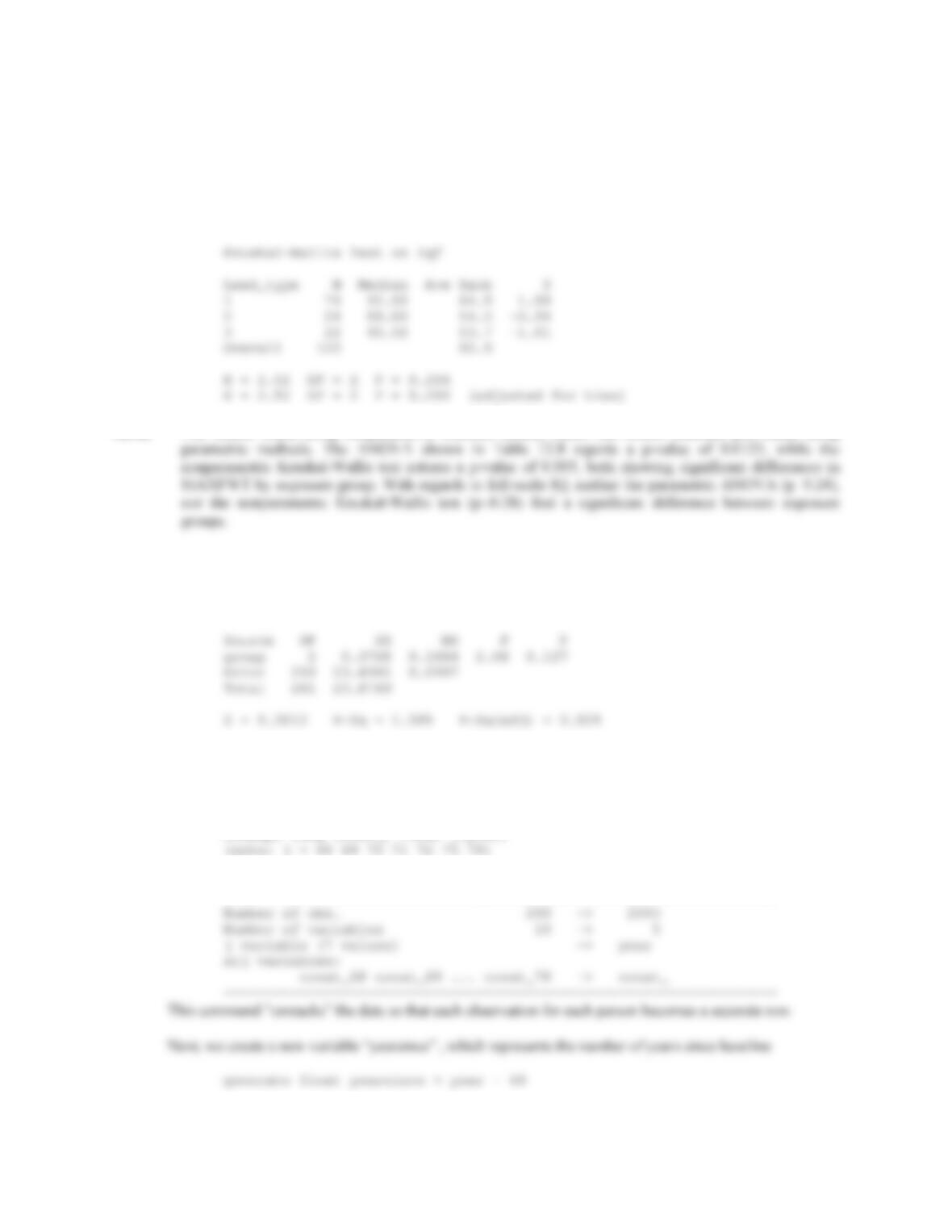
12.44 Using the Kruskal-Wallis test, we find significant differences in the finger-tapping variable MAXFWT,
by exposure group, with a p-value 0.005
Kruskal-Wallis Test: MAXFWT versus Lead_type
CHAPTER 12/MULTISAMPLE INFERENCE 340
12.45 We do not find a difference in full-scale IQ between exposure groups (p=0.28), though we do note that
the unexposed group shows the largest median IQ, while the currently-exposed group shows the lowest
median IQ.
Kruskal-Wallis Test: Iqf versus Lead_type
120 cases were used
4 cases contained missing values
12.46 The results found using nonparametric methods closely match the results obtained previously using
12.47 After creating our response variable, CreChange = “creat_78 – creat_68”, we perform a one-way
ANOVA, and find no significant difference in serum-creatinine changes between the three groups.
One-way ANOVA: CreChange versus group
12.48-12.51
For these problems, we need to use STATA to reshape our data set. If we use the following coding, we can
more easily perform the required analysis. First, we should remove the one person who has only a single
observation, as no regression model can be fit to a single point.
reshape long creat_, i(id) j(year)
Data wide -> long
——————————————————————