Accounting Chapter 11 Homework We will repeat the analyses with those points removed

288 CHAPTER 11/REGRESSION AND CORRELATION METHODS

Regression Analysis: SaltInd2 versus Mn_sbp

The regression equation is

SaltInd2 = – 10.3 + 0.108 Mn_sbp

Regression Analysis: SugarInd versus Mn_sbp

The regression equation is

SugarInd = – 34.6 + 0.580 Mn_sbp

4

3

Residuals Versus Mn_sbp

(response is SaltInd1)

3

2

Residuals Versus Mn_sbp

(response is SaltInd2)

1009080706050

-5.0

Mn_sbp

CHAPTER 11/REGRESSION AND CORRELATION METHODS 289

Regression Analysis: SaltInd1 versus Mn_sbp

The regression equation is

Regression Analysis: SugarInd versus Mn_sbp

The regression equation is

11.45 We perform a similar analysis to that in 11.42, this time using DBP as our explanatory variable. For the

“salt index 1” and “sugar index”, we will continue to keep the previously identified outliers out of the

analyses. Significant p-values are bolded and underlined.

Regression Analysis: SaltInd1 versus Mn_dbp

The regression equation is

Regression Analysis: SaltInd2 versus Mn_dbp

Regression Analysis: SugarInd versus Mn_dbp

The regression equation is

SugarInd = – 18.9 + 0.592 Mn_dbp

290 CHAPTER 11/REGRESSION AND CORRELATION METHODS

S = 18.9820 R-Sq = 4.9% R-Sq(adj) = 3.9%

2

Residuals Versus Mn_dbp

(response is SaltInd1)

4

3

Residuals Versus Mn_dbp

(response is SaltInd2)

11.46 For this exercise, we omit all entries which contain “lead type” = 3. When we fit our regression model,

we find no significant effect of age, gender, or lead exposure on IQF.

Regression Analysis: Iqf_0 versus Lead_type_0, Age_0, Sex_0

6560555045403530

-3

Mn_dbp

CHAPTER 11/REGRESSION AND CORRELATION METHODS 291

Our residual plot shows some evidence of non-constant variance, so we will refit the model using sqrt(IQF)

as the response variable.

This new model still shows no significant relationship between lead exposure and IQF, and we still see

evidence of non-constant variance. (Note: using ln(IQF) as the response variable produces similar results)

1600140012001000800600400200

3

-3

-4

Age_0

Residuals Versus Age_0

(response is rtIQF)

11.47 Previously, we have defined MAXFWT to be the maximum of FWT_r and FWT_l for each child. We

will regress the value MAXFWT on blood level, age, and sex. It is important to remember that missing

values are coded as “99” in this data set, and to make sure not include these values in the analysis.

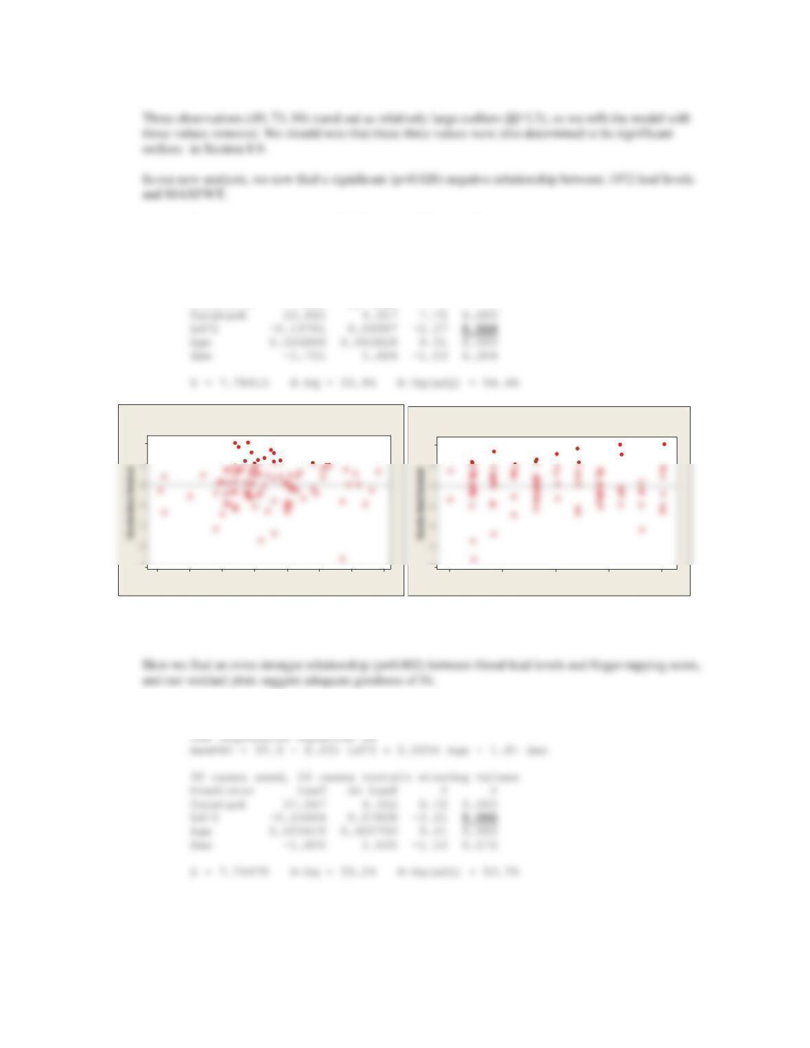
Our initial regression model using 1972 lead levels finds age alone to be significantly related to

MAXFWT.

The regression equation is

150012501000750500

4

3

-4

Age

Residuals Versus Age

(response is maxFWT)

706050403020100

4

3

2

-4

Ld72

Residuals Versus Ld72

(response is maxFWT)

292 CHAPTER 11/REGRESSION AND CORRELATION METHODS

Regression Analysis: maxFWT versus Ld72, Age, Sex

The regression equation is

maxFWT = 33.5 – 0.138 Ld72 + 0.0269 Age – 1.72 Sex

92 cases used, 32 cases contain missing values

Predictor Coef SE Coef T P

706050403020100

2

-4

Ld72

Residuals Versus Ld72

(response is maxFWT)

150012501000750500

2

-4

Age

Residuals Versus Age

(response is maxFWT)

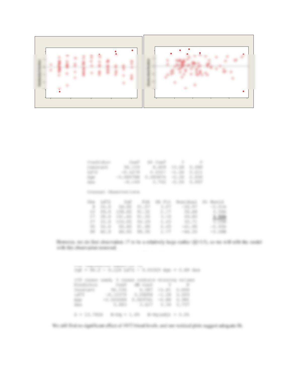
We will repeat the analysis, but use 1973 lead levels instead, while still keeping the 3 outliers out of the

data set.

Regression Analysis: maxFWT versus Ld73, Age, Sex

CHAPTER 11/REGRESSION AND CORRELATION METHODS 293

150012501000750500

2

-3

-4

Age

Residuals Versus Age

(response is maxFWT)

605040302010

2

-3

-4

Ld73

Residuals Versus Ld73

(response is maxFWT)

11.48 In the initial model, we find no significant relationship between 1972 lead levels and IQF.

Regression Analysis: Iqf versus Ld72, Age, Sex

The regression equation is

Iqf = 96.1 – 0.128 Ld72 – 0.00079 Age – 0.15 Sex

121 cases used, 3 cases contain missing values

Regression Analysis: Iqf versus Ld72, Age, Sex

294 CHAPTER 11/REGRESSION AND CORRELATION METHODS

3

2

Residuals Versus Age

(response is Iqf)

3

2

Residuals Versus Ld72

(response is Iqf)

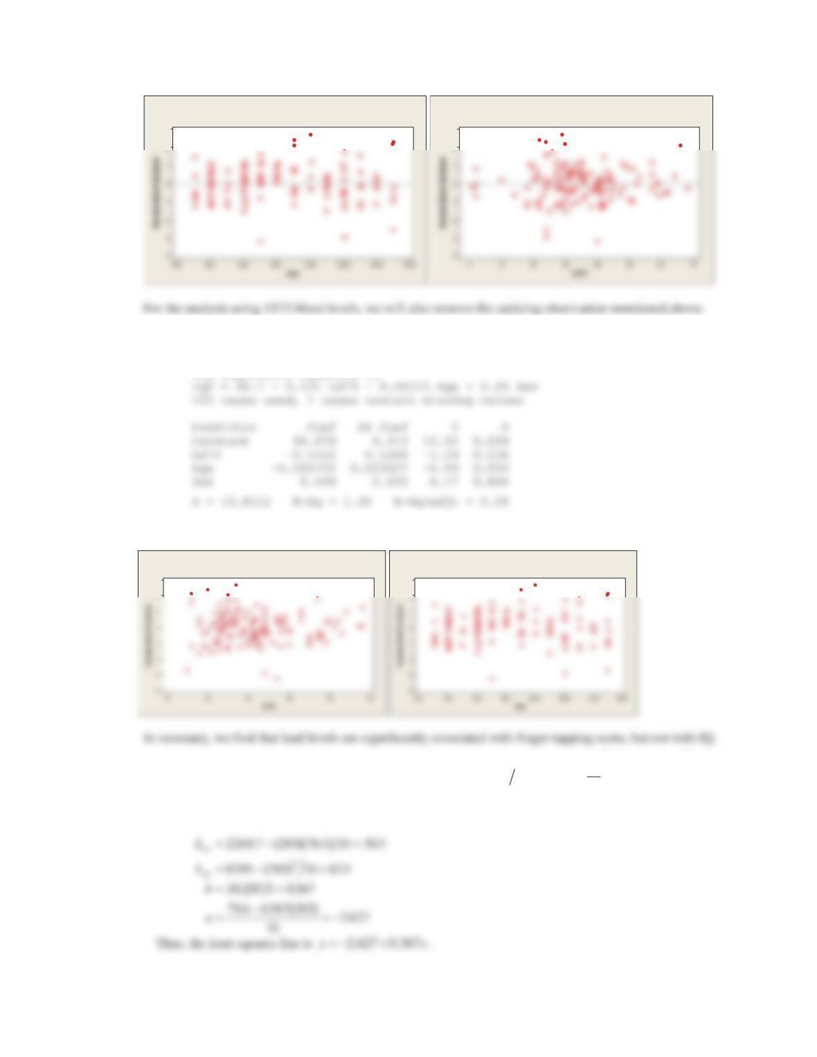
Again, we find no significant associations between any covariates and IQF.

Regression Analysis: Iqf versus Ld73, Age, Sex

The regression equation is

Our residual plots suggest adequate fit.

3

Residuals Versus Ld73

(response is Iqf)

3

Residuals Versus Age

(response is Iqf)

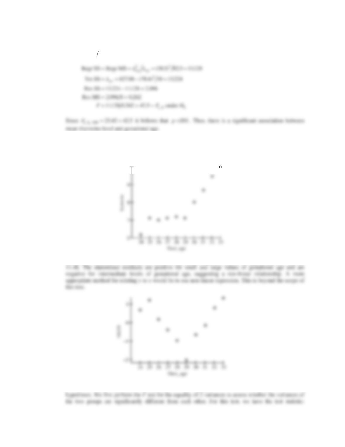
11.49 We fit the least squares line given by yabx  , where bL L

xy xx

and

a 1

10 y

i

bx

i

i 1

10

¦

i 1

10

¦

§

©

¨

·

¹

¸

. We

have that

CHAPTER 11/REGRESSION AND CORRELATION METHODS 295

11.50 We wish to test the hypothesis :

E

0 vs. : . We use the test statistic

under . In this example,

11.51 We plot the mean thyroxine level vs gestational age below. The relationship does not look very linear

with the average thyroxine level relatively constant for gestational ages of 24–29 weeks and then linearly

increasing after 29 weeks.

10

We also have plotted the studentized residuals vs gestational age from the linear regression fit in Problem

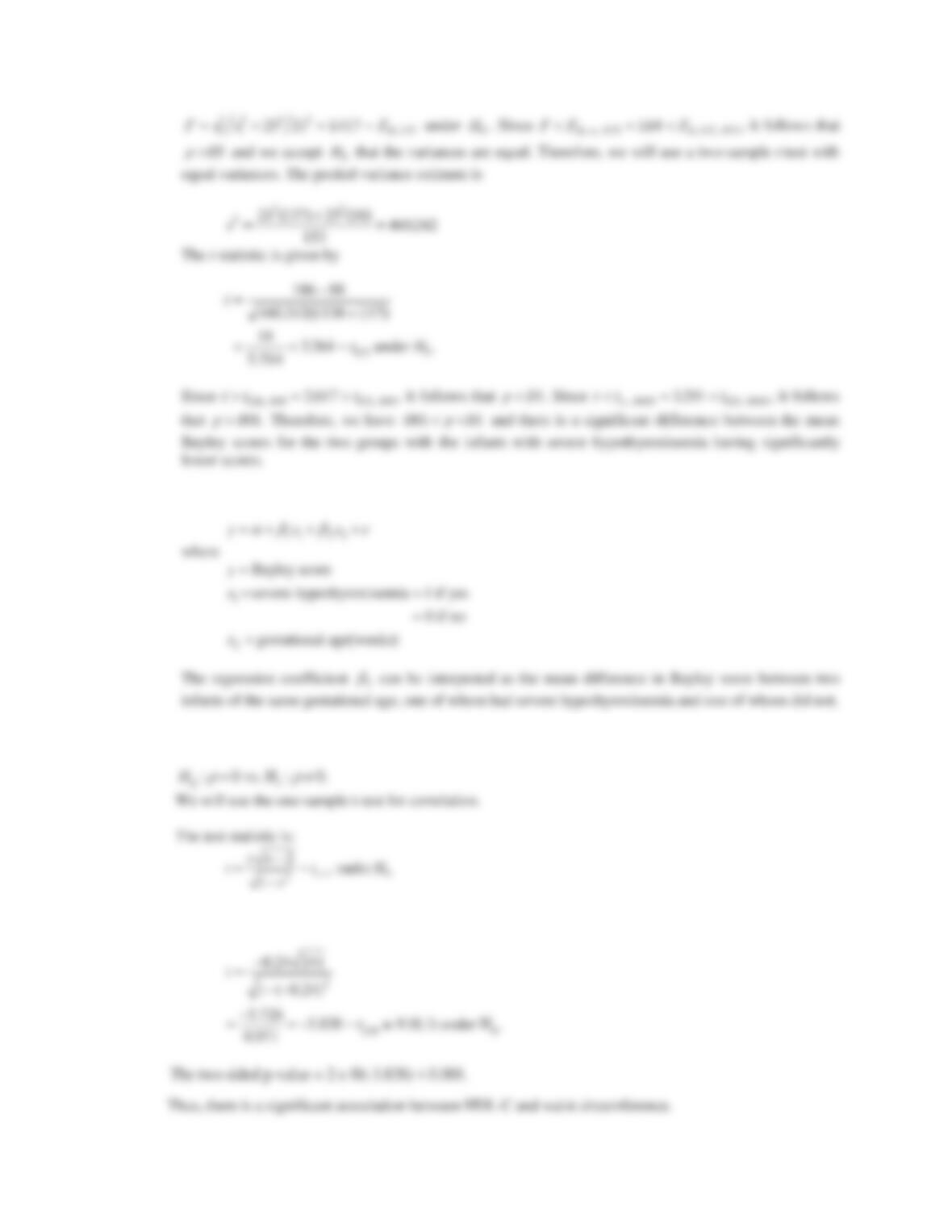
11.52 We wish to test the hypothesis : vs. : . We will use a two-sample t test to these

H0H1

E

z0

F

Regr MS Res MS

~

,18 H0

H0

P

12

H1

P

12

z

296 CHAPTER 11/REGRESSION AND CORRELATION METHODS

11.53 We can use the multiple regression model

11.54 We wish to test the hypothesis:

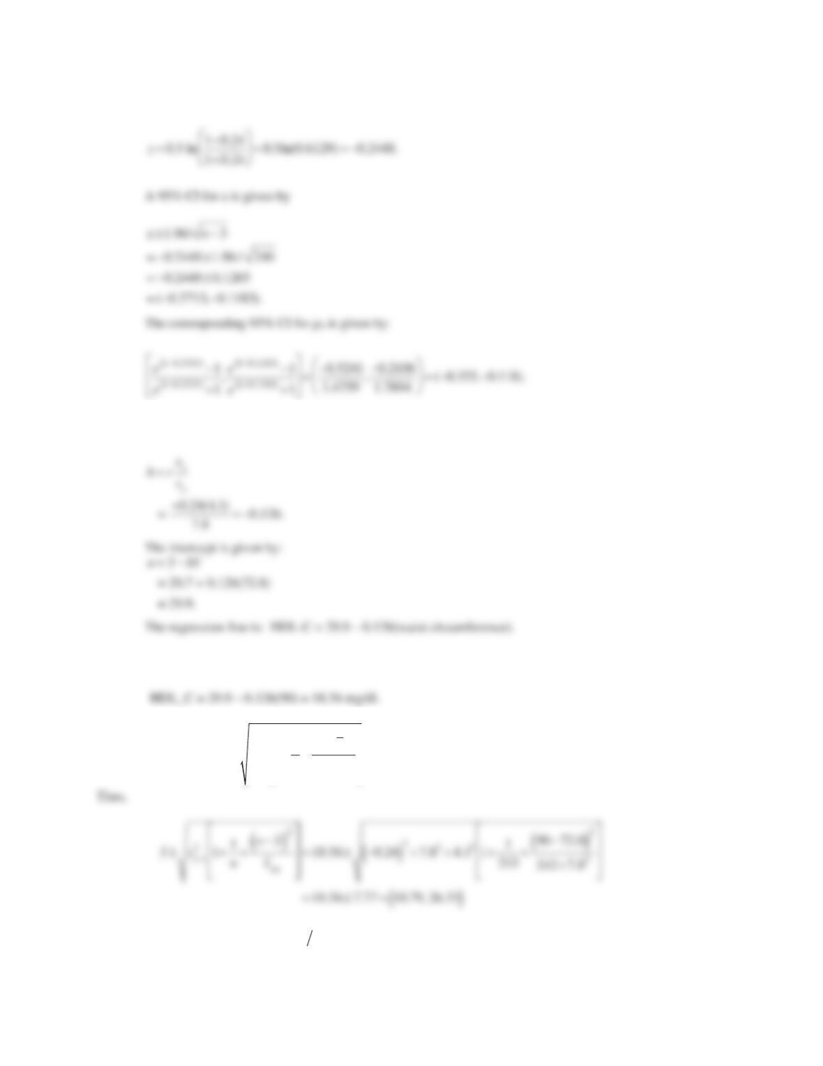
11.55 The test statistic is

CHAPTER 11/REGRESSION AND CORRELATION METHODS 297

11.56 We use the Fisher’s z transformation approach. The z statistic is given by



11.57 The relationship between a regression coefficient and a correlation coefficient is given by:

11.58 The expected HDL-C for an average person with wait circumference = 90 cm is

11.59 The 95% CI is

ˆ

yrs

y.x

2

11

nxx



2

L

xx

ª

¬

«

º

¼

»

where

s

y.x

rus

x

us

y

and L

xx

(n1)s

x

2

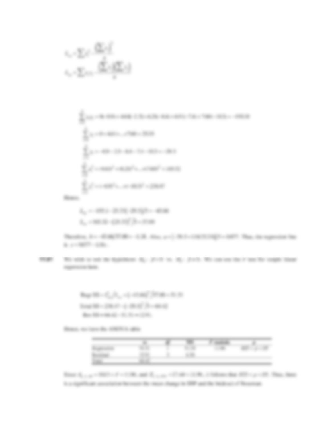
11.60 We use the formula , where

bL L

xy xx

298 CHAPTER 11/REGRESSION AND CORRELATION METHODS

We have

11.62 We have

CHAPTER 11/REGRESSION AND CORRELATION METHODS 299

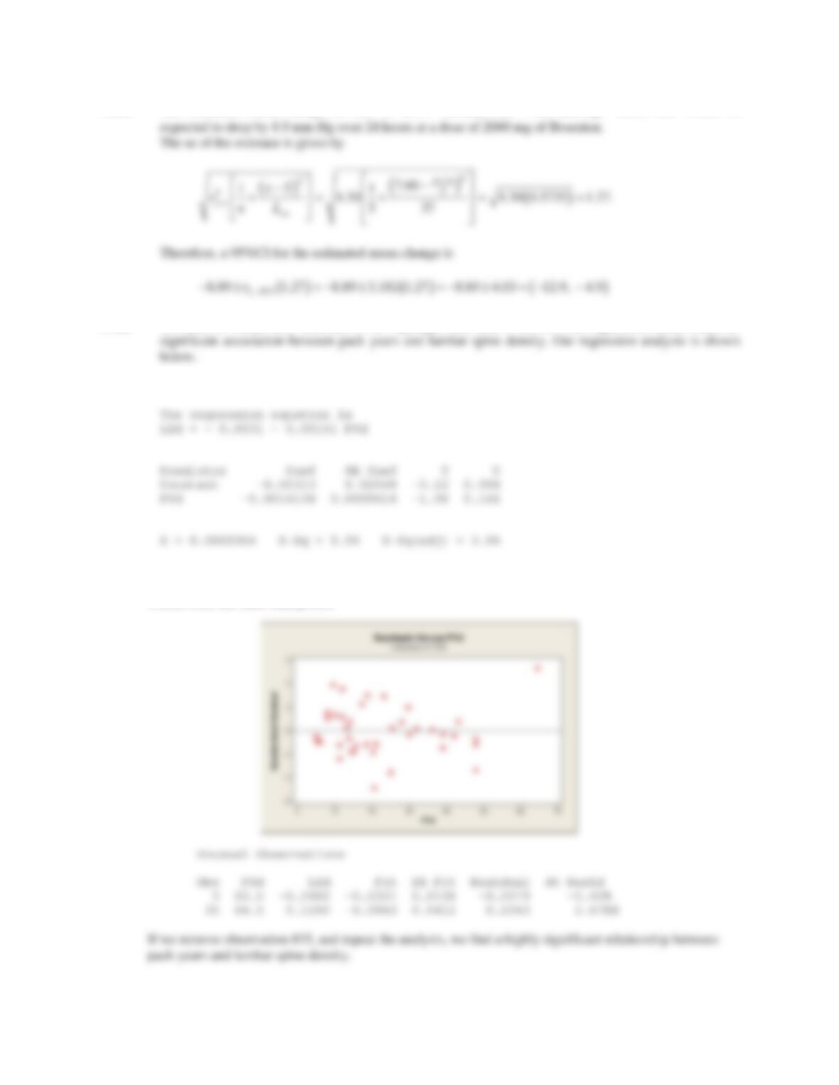
11.63 The estimated mean change in SBP is . Thus, SBP would be

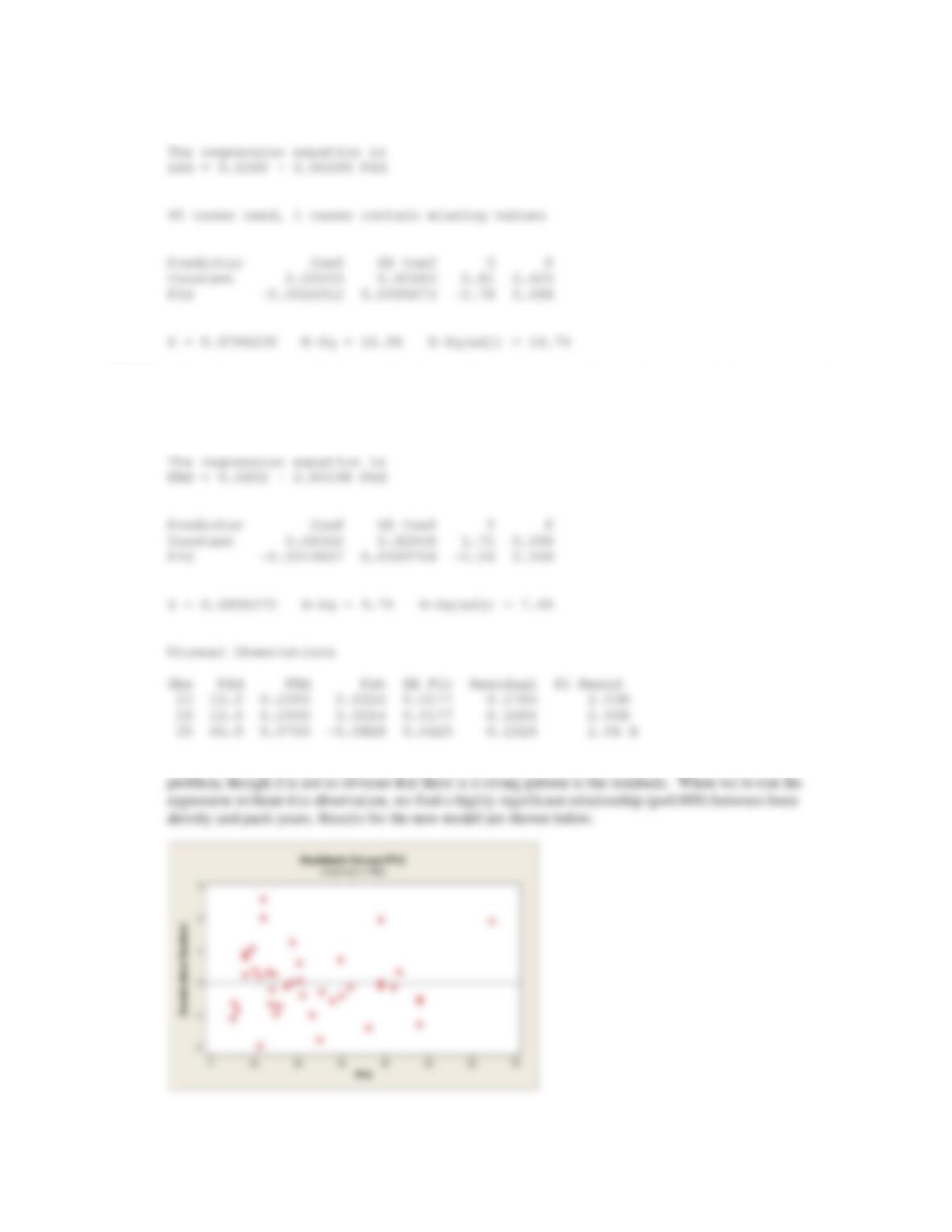
11.64 We need to create new variables PYd = py2-py1 and LSd = ls2-ls1. Our regression model finds no

Regression Analysis: LSd versus PYd

To assess goodness of fit, we show the studentized residuals. There seems to be a general negative trend in

the residuals that is offset by observation 35, which is a fairly large positive outlier, and is far away (on the

x-axis) from the other data points.

0 077 118 2000 889..ln .





 mm Hg

300 CHAPTER 11/REGRESSION AND CORRELATION METHODS

Regression Analysis: LSd versus PYd

11.65 For this analysis, we find a moderately significant association between femoral neck density and pack-

years smoked. Regression output from MINITAB is shown below.

Regression Analysis: FNd versus PYd

MINITAB finds three moderate outliers, including observation #35, which we found in the previous

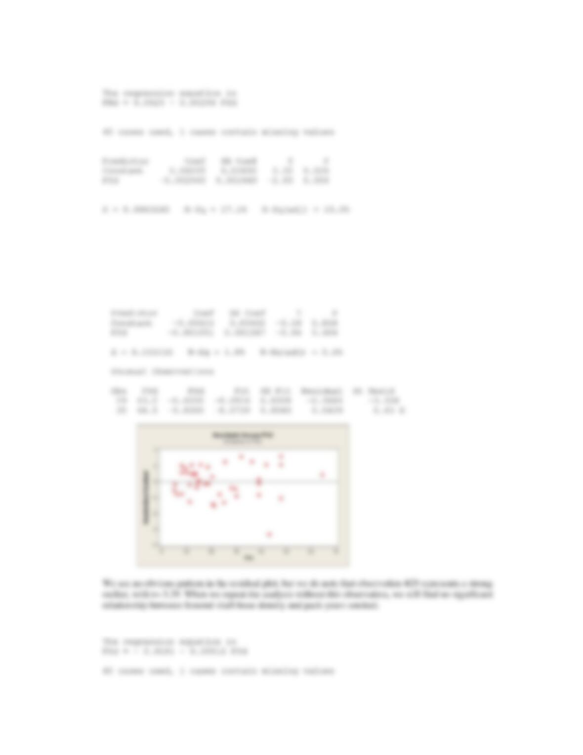
CHAPTER 11/REGRESSION AND CORRELATION METHODS 301

Regression Analysis: FNd versus PYd

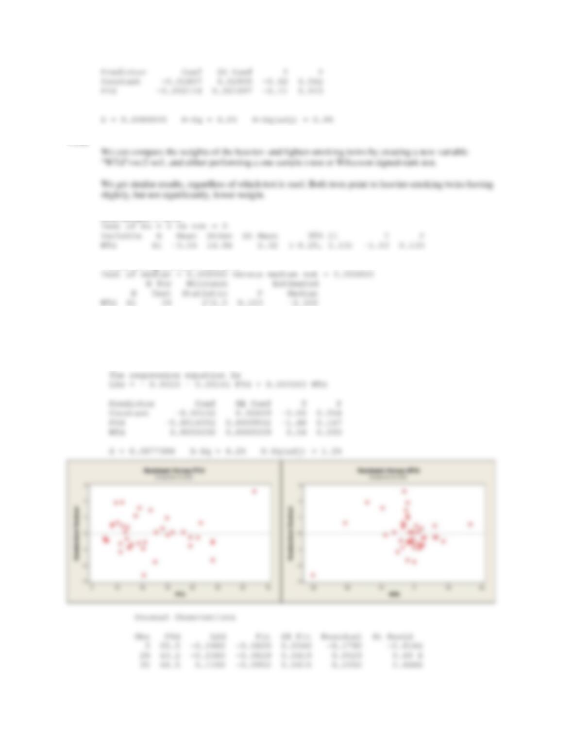
11.66 When we look at femoral shaft bone density, we find no significant relationship with pack-years

smoked.

Regression Analysis: FSd versus PYd

The regression equation is

FSd = – 0.0061 – 0.00105 PYd

Regression Analysis: FSd versus PYd

302 CHAPTER 11/REGRESSION AND CORRELATION METHODS

11.67

One-Sample T: WTd

Wilcoxon Signed Rank Test: WTd

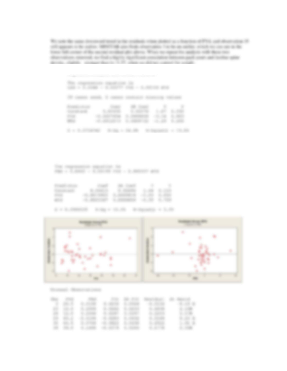
11.68 When we regress the difference in lumbar spine density LSd on both WTd and PYd, we find no

significant association between pack years smoked and lumbar spine density, after controlling for weight.

Regression Analysis: LSd versus PYd, WTd

CHAPTER 11/REGRESSION AND CORRELATION METHODS 303

density, slightly stronger than in 11.57, when we did not control for weight.

Regression Analysis: LSd versus PYd, WTd

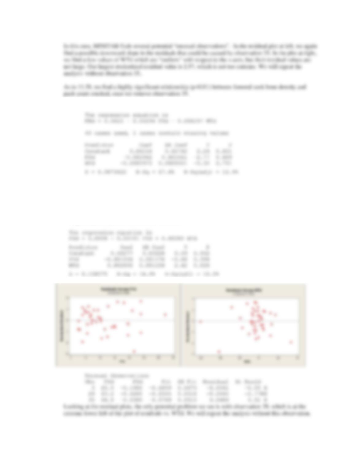
11.69 As in 11.58, our initial regression model finds a barely significant (p=0.050) association between femoral

neck bone density and pack-years.

Regression Analysis: FNd versus PYd, WTd

304 CHAPTER 11/REGRESSION AND CORRELATION METHODS

Regression Analysis: FNd versus PYd, WTd

11.70 When we look at femoral shaft bone density while controlling for weight, we still find no significant

relationship with pack-years smoked. However, we do find that weight is significantly related to bone

density.

Residuals from FNd vs WTd

Regression Analysis: FSd versus PYd, WTd

CHAPTER 11/REGRESSION AND CORRELATION METHODS 305

After removing this observation, we find no significant association between femoral shaft density and

weight or pack-years smoked.

Regression Analysis: FSd versus PYd, WTd

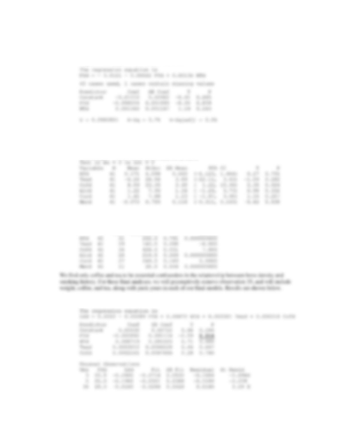
11.71 After creating difference variables for each of the possible confounders (height, tea, coffee, alcohol,

current smoking, and menopause status), we can again perform t-tests and/or signed-rank tests for each

variable to see if there is any relationship between the variables and smoking history.

One-Sample T: HTd, Tead, Cofd, Alcd, Curd, Mend

Wilcoxon Signed Rank Test: HTd, Tead, Cofd, Alcd, Curd, Mend

Test of median = 0.000000 versus median not = 0.000000

N for Wilcoxon Estimated

N Test Statistic P Median

Regression Analysis: LSd versus PYd, WTd, Tead, Cofd