268
REGRESSION AND
CORRELATION
METHODS
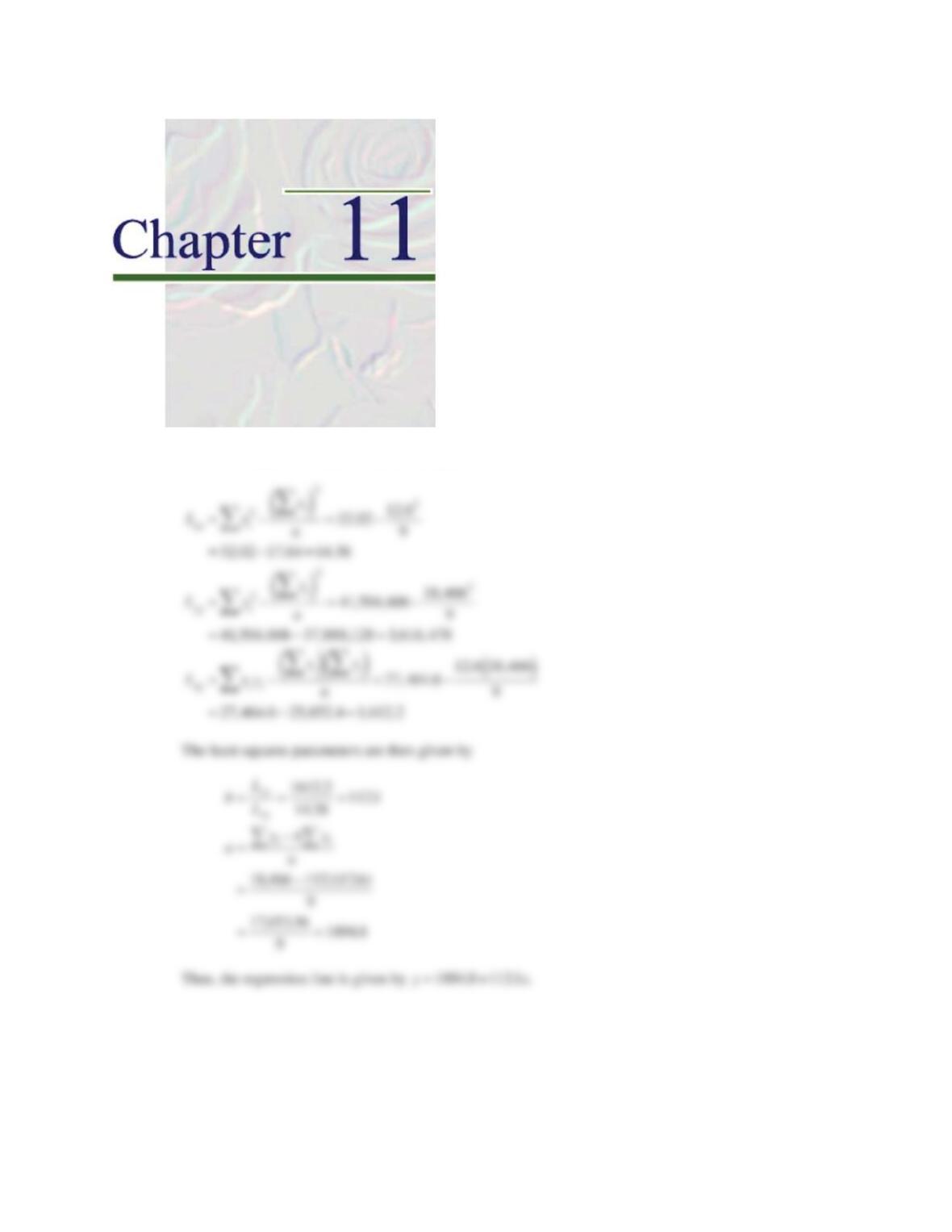
11.1 We first compute the sums of squares and products as follows
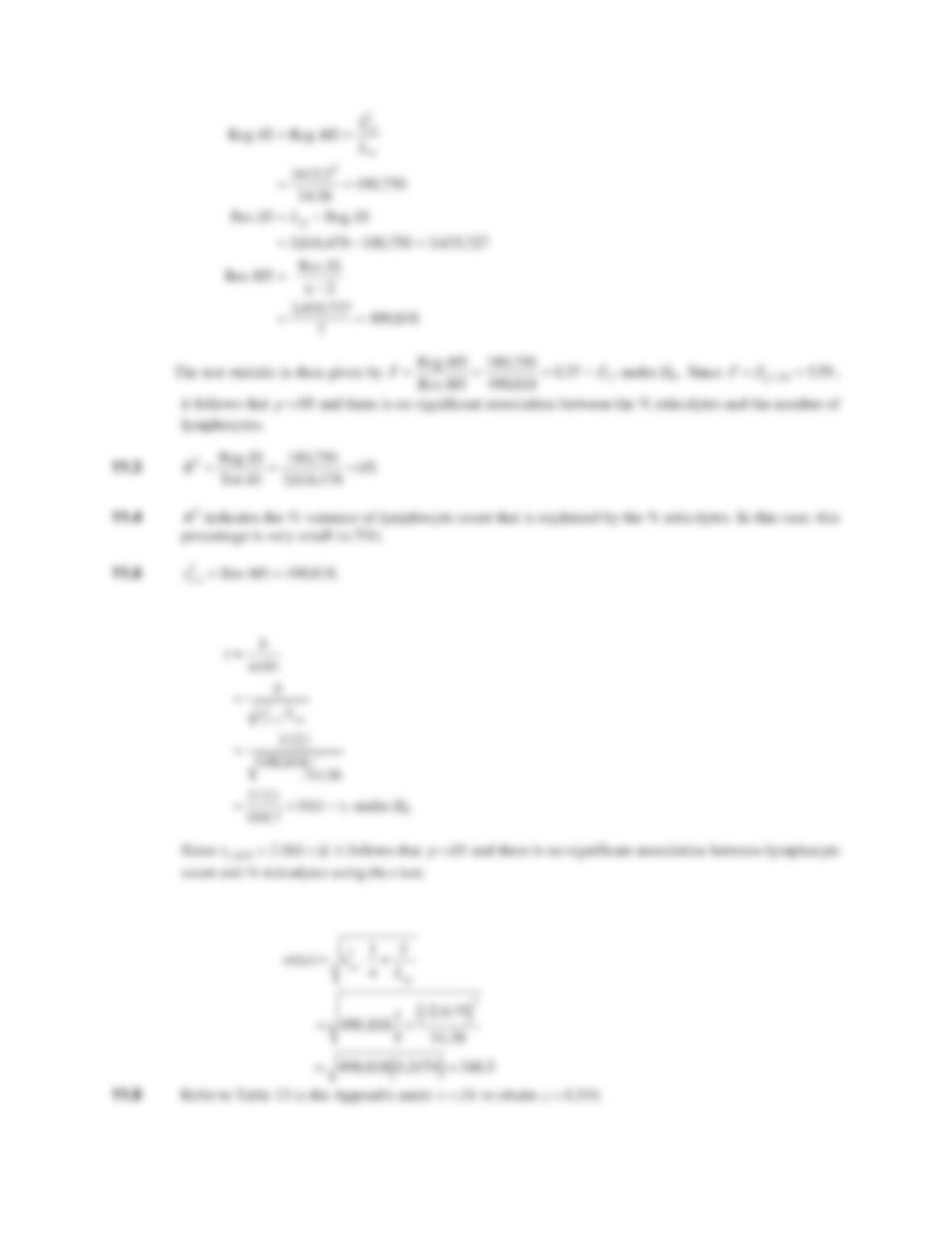
11.2 We compute the Regression and Residual sums of squares and mean squares as follows
CHAPTER 11/REGRESSION AND CORRELATION METHODS 269
11.6 We have the test statistic
11.7 From Problem 11.6, Furthermore, we have
s
eb
184 7..
270 CHAPTER 11/REGRESSION AND CORRELATION METHODS
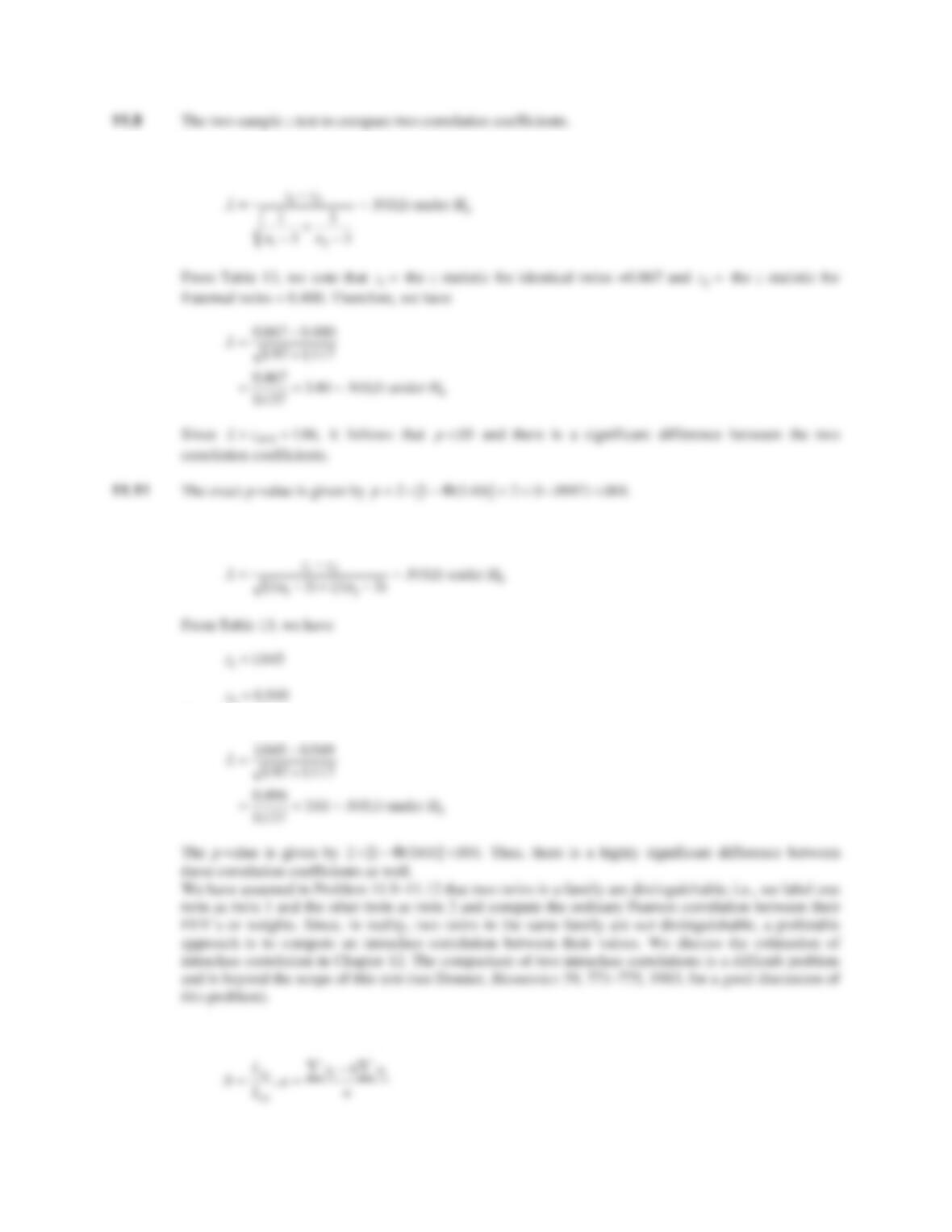
11.10 We wish to test the hypothesis . We use the test statistic
11.12 We have the test statistic
Thus,
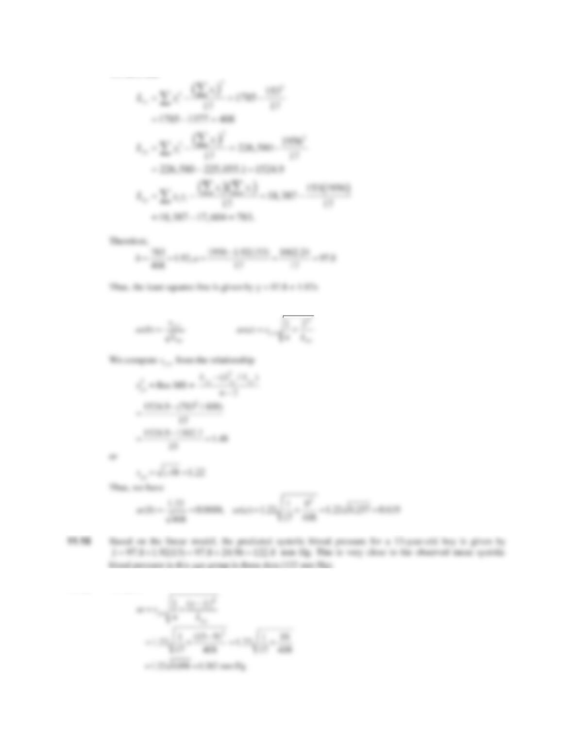
11.13 The least squares estimates are given by
H
H
01 2 11 2
::
U
U
U
U
zvs
20 549 .
CHAPTER 11/REGRESSION AND CORRELATION METHODS 271
We have that
11.14 The standard errors of the regression parameters are given by
11.16 We have
272 CHAPTER 11/REGRESSION AND CORRELATION METHODS
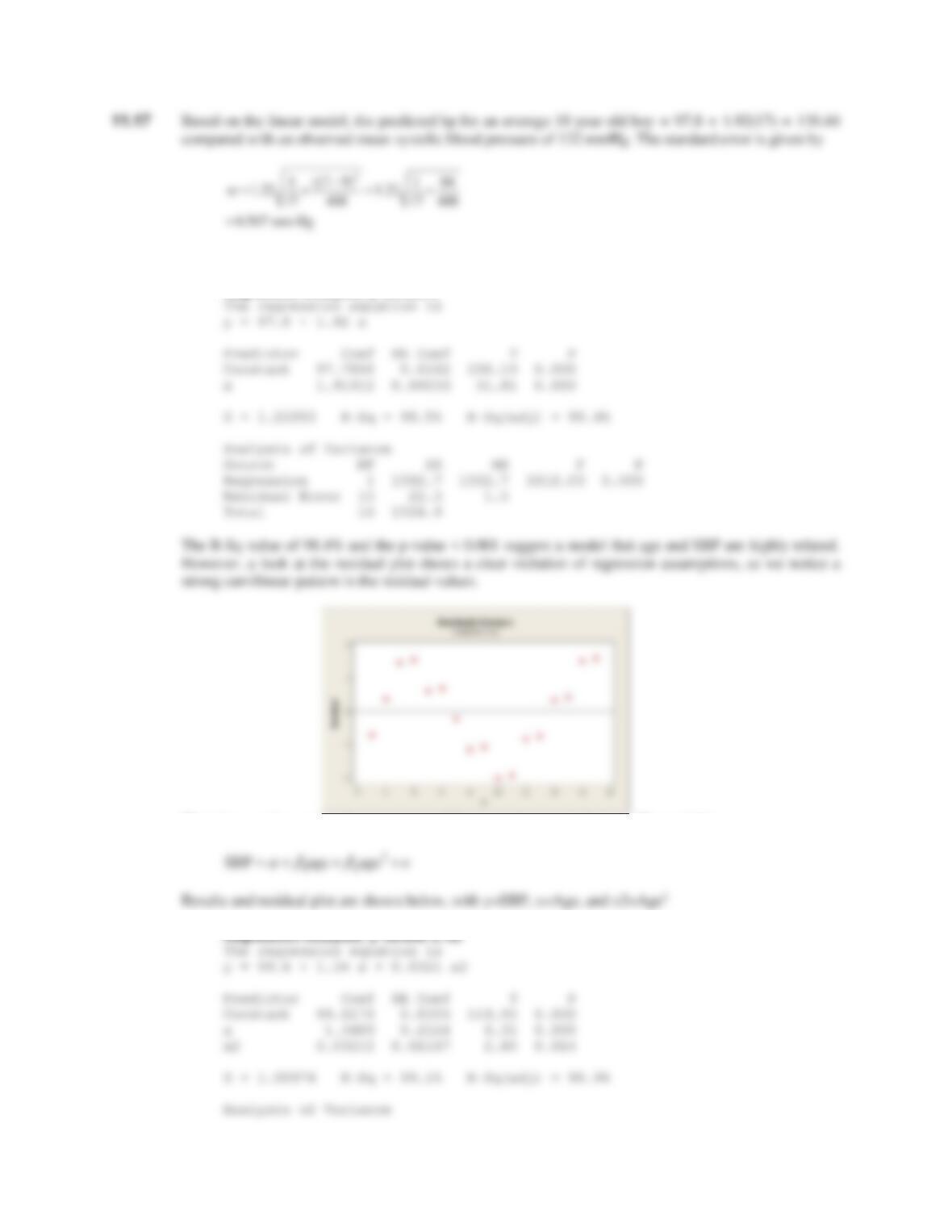
11.18 We have run the regression using MINITAB as shown below, where y=SBP and x=Age.
Regression Analysis: y versus x
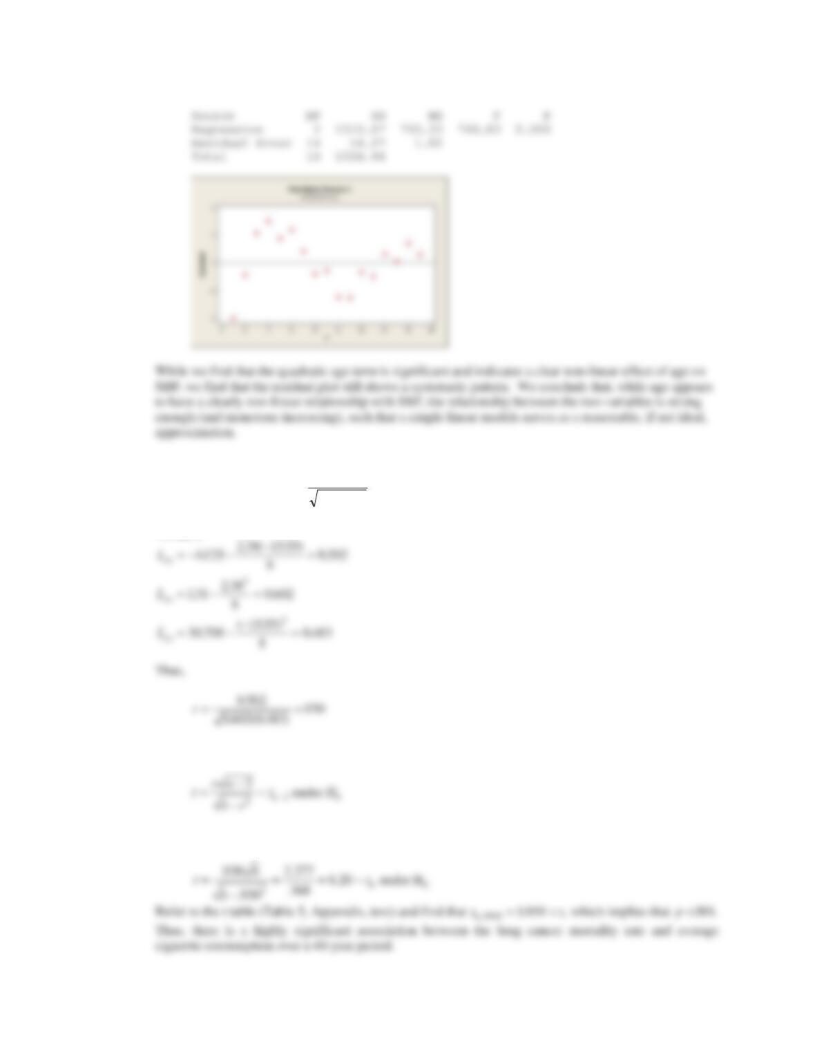
Therefore, we have rerun the regression adding a quadratic term for age. The model is
CHAPTER 11/REGRESSION AND CORRELATION METHODS 273
11.19 The correlation is given by
We have
11.20 Use the test statistic
In this case
rL
LL
xy
xx yy
u
274 CHAPTER 11/REGRESSION AND CORRELATION METHODS
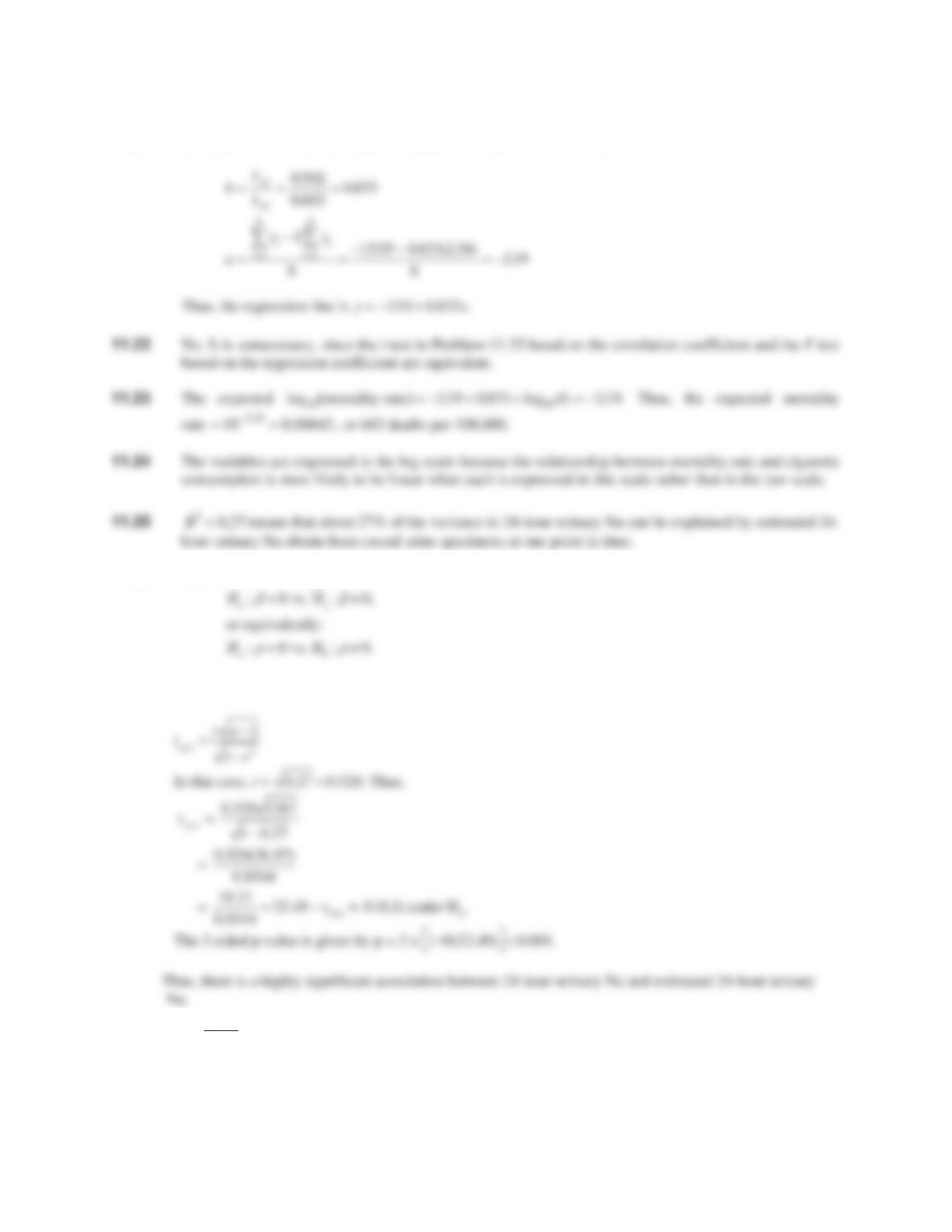
11.21 It is also of interest to fit a regression line to these data of the form where
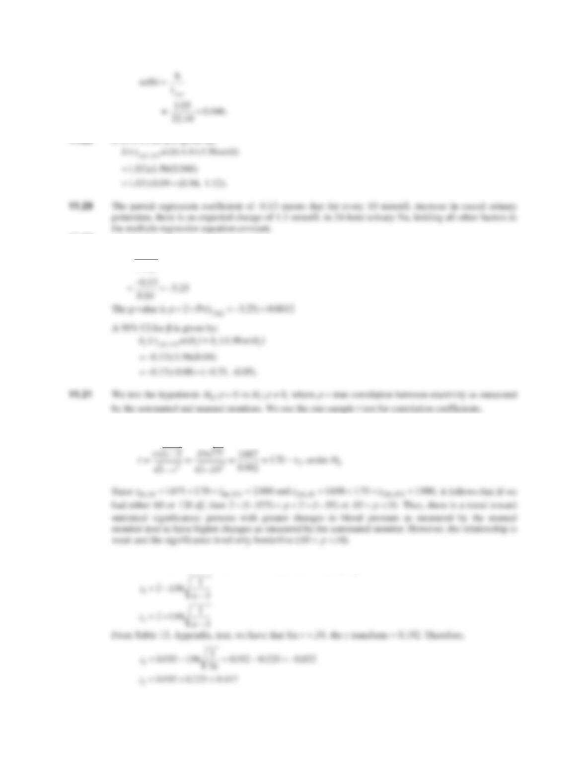
11.26 We wish to test the hypothesis:
We use the one-sample t-test for correlation given by:
11.27
t
reg
b
se(b) t
corr
.
Thus,
yabx ,
CHAPTER 11/REGRESSION AND CORRELATION METHODS 275
11.28 A 95% CI for ȕ is given by:
11.30
t
reg
b
l
se(b
)
11.32 The test statistic is
11.33 A 95% CI for z (the Fisher’s z transform of
U
) is given by
z
1
,z
2
,
where
276 CHAPTER 11/REGRESSION AND CORRELATION METHODS
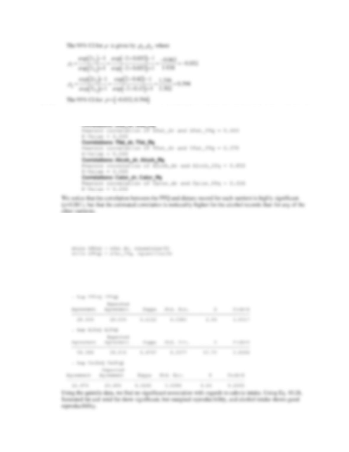
11.34 If we use the continuous data, we can use MINITAB to estimate the correlation between each pair of
intake records, as shown below:
` To use the quintile data, we will use STATA, with the code below showing how to convert and store
continuous data as quintile values. We then use the Kappa statistic from Chapter 10 to assess
reproducibility. Results are shown below.
. kap SfDrQ SfFqQ
Expected
Agreement Agreement Kappa Std. Err. Z Prob>Z
—————————————————————–
31.79% 20.01% 0.1473 0.0380 3.88 0.0001
CHAPTER 11/REGRESSION AND CORRELATION METHODS 277
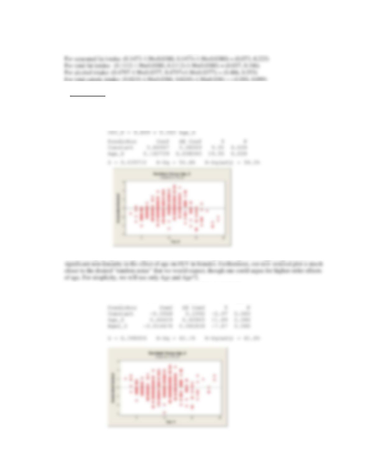
11.35 The 95% confidence interval is given by
N
r1.96se
N
. Therefore, we have
For total caloric intake: (0.0245-1.96×0.0380, 0.0245+1.96×0.038) = (-0.050, 0.099)
11.36 Females only:
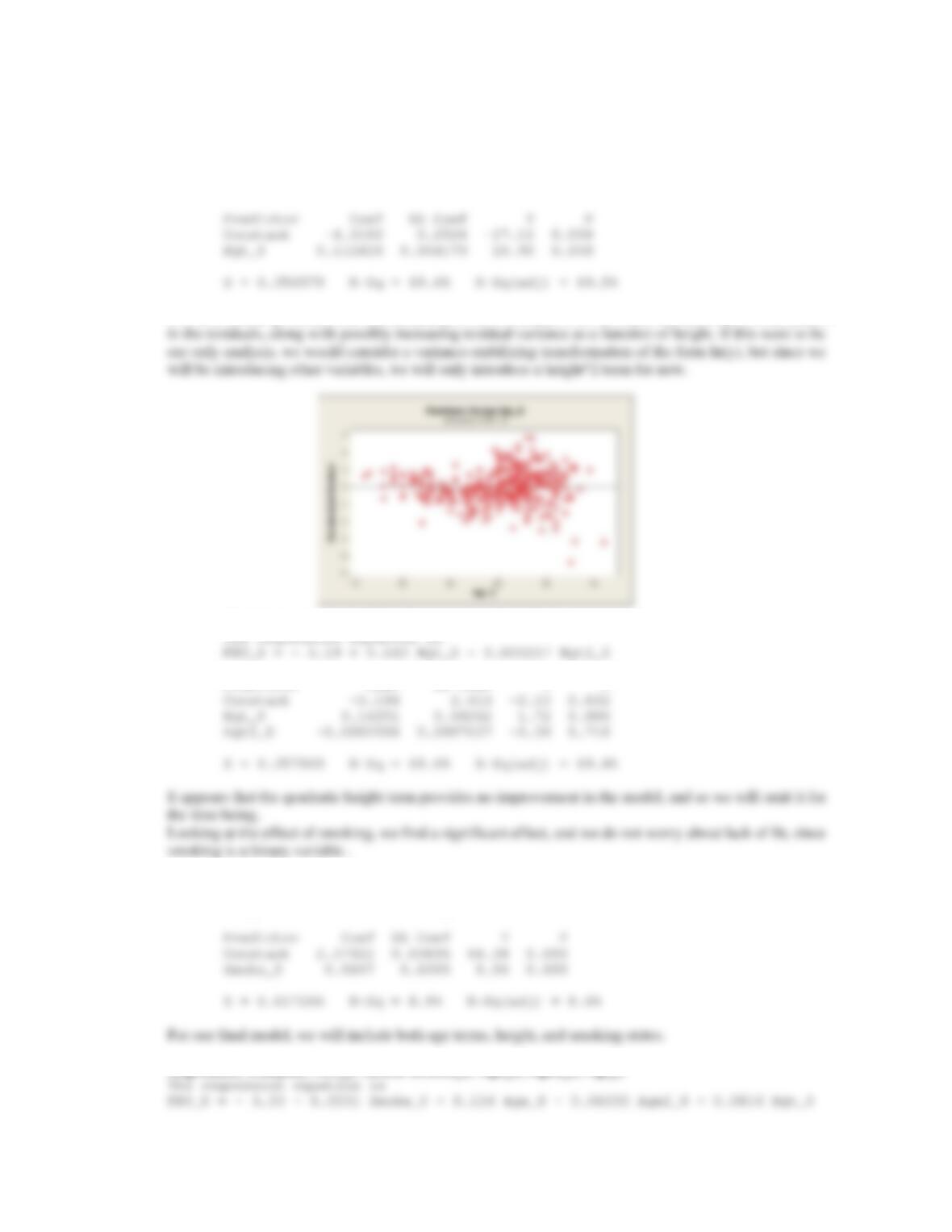
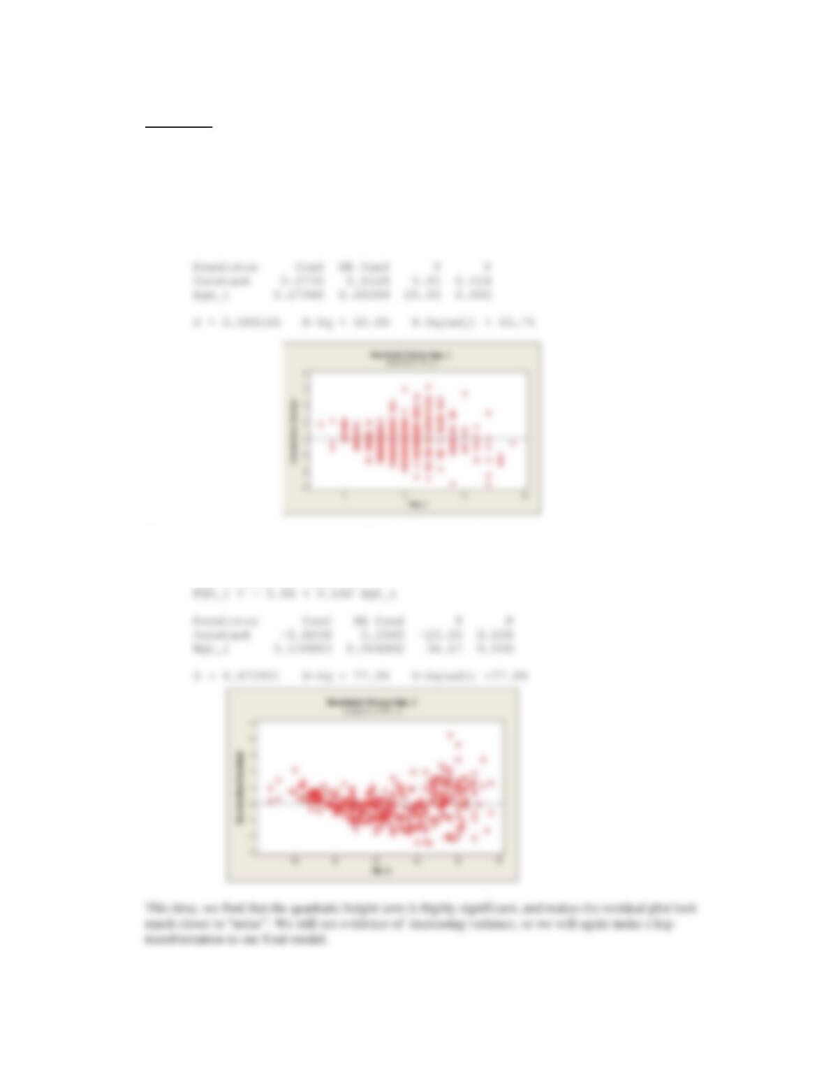
First, we look at the effect of age. We find a highly significant relationship, but we notice a strong
quadratic shape in the residual plot, leading us consider the addition of an Age^2 term.
Regression Analysis: FEV_0 versus Age_0
The regression equation is
We find a highly significant p-value associated with the new quadratic age term, suggesting that there is
Regression Analysis: FEV_0 versus Age_0, Age2_0
The regression equation is
FEV_0 = – 0.592 + 0.464 Age_0 – 0.0145 Age2_0
278 CHAPTER 11/REGRESSION AND CORRELATION METHODS
When we regress FEV on height, we also find a highly significant relationship, with p<0.001
Regression Analysis: FEV_0 versus Hgt_0
The regression equation is
FEV_0 = – 4.32 + 0.112 Hgt_0
We have similar problems with the residual plot for this analysis, as we notice a distinct curvilinear pattern
Regression Analysis: FEV_0 versus Hgt_0, Hgt2_0
Predictor Coef SE Coef T P
Regression Analysis: FEV_0 versus Smoke_0
The regression equation is
FEV_0 = 2.38 + 0.587 Smoke_0
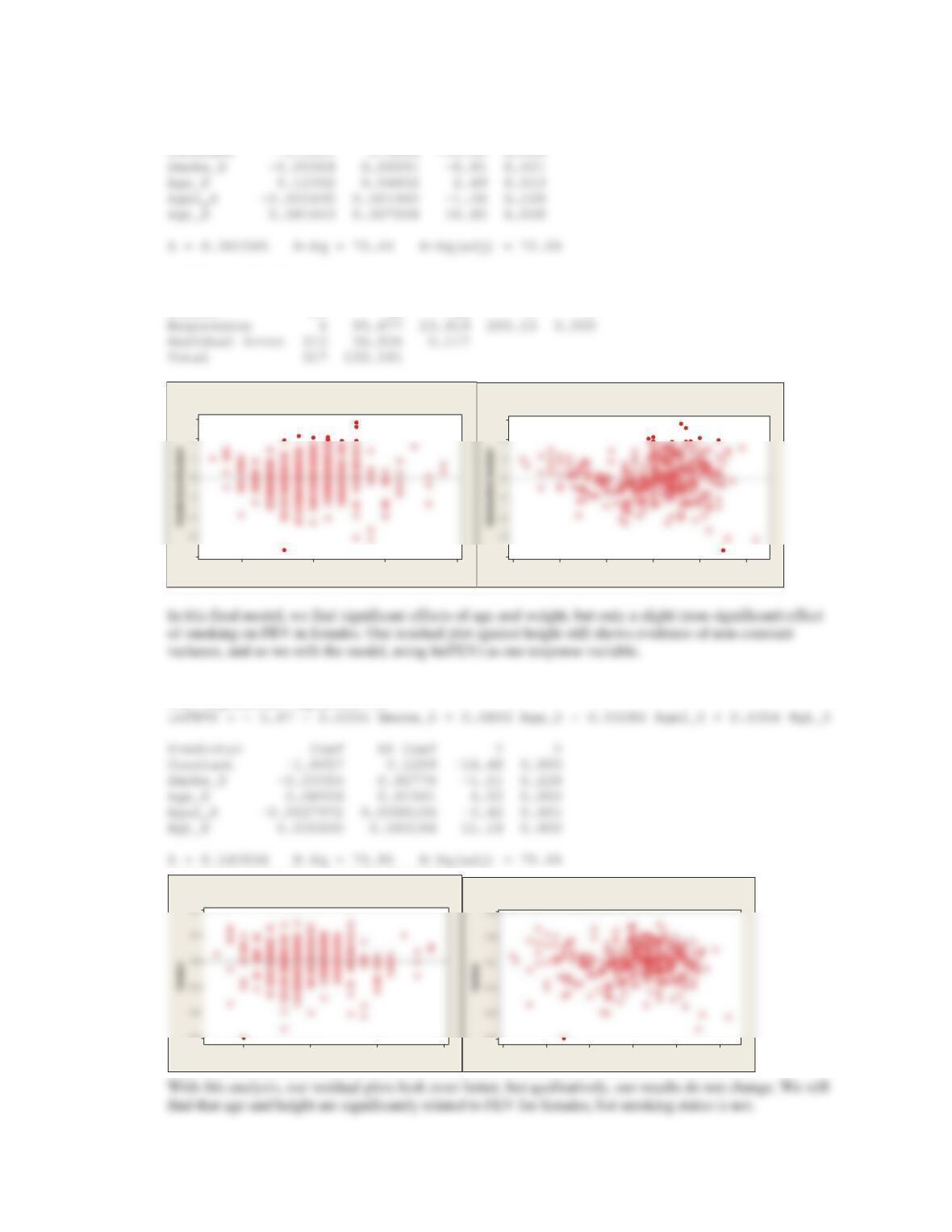
Regression Analysis: FEV_0 versus Smoke_0, Age_0, Age2_0, Hgt_0
CHAPTER 11/REGRESSION AND CORRELATION METHODS 279
Predictor Coef SE Coef T P
Analysis of Variance
Source DF SS MS F P
2015105
3
-4
Age_0
Residuals Versus Age_0
(response is FEV_0)
706560555045
3
-4
Hgt _ 0
Residuals Versus Hgt_0
(response is FEV_0)
Regression Analysis: lnFEV0 versus Smoke_0, Age_0, Age2_0, Hgt_0
The regression equation is
2015105
-0.6
Age_0
Residuals Versus Age_0
(response is lnFEV0)
706560555045
-0.6
Hgt_0
Residuals Versus Hgt_0
(response is lnFEV0)
280 CHAPTER 11/REGRESSION AND CORRELATION METHODS
Males only:
Unlike the female-only analysis, we do not see an obvious need to extend beyond a linear effect of age. The
linear term is highly significant, and we do not detect departures from normality in the residual plot. It does
appear that variance may be increasing with age, so we will again consider a transformation for our final
model.
Regression Analysis: FEV_1 versus Age_1
The regression equation is
FEV_1 = 0.074 + 0.273 Age_1
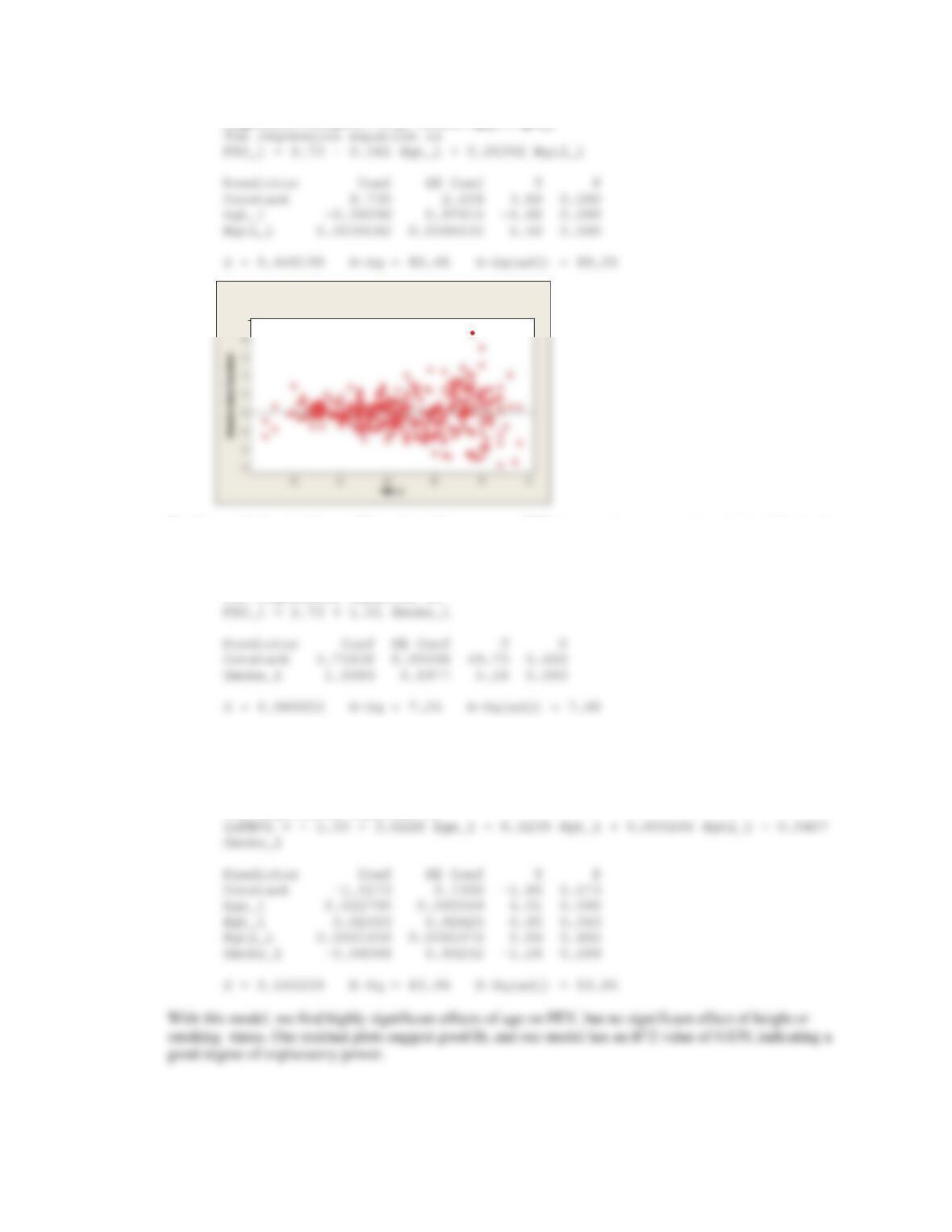
When looking at the effect of height on FEV, we again find a strong relationship, with a residual plot that
leads us to refit the model with a quadratic term.
The regression equation is
CHAPTER 11/REGRESSION AND CORRELATION METHODS 281
Regression Analysis: FEV_1 versus Hgt_1, Hgt2_1
Finally, we find a significant effect of smoking status on FEV, but we do not worry about lack of fit, for the
same reasons described above.
Regression Analysis: FEV_1 versus Smoke_1
The regression equation is
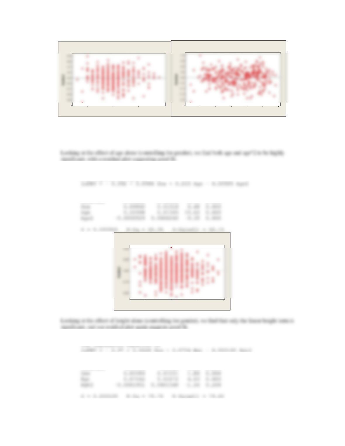
For our final model, we will use ln(FEV) as the response variable, and include Age, Height, Height^2, and
smoking status.
Regression Analysis: lnFEV1 versus Age_1, Hgt_1, Hgt2_1, Smoke_1
The regression equation is
5
Residuals Versus Hgt_1
(response is FEV_1)
282 CHAPTER 11/REGRESSION AND CORRELATION METHODS
2015105
-0.5
Age_1
Residuals Versus Age_1
(response is lnFEV1)
757065605550
-0.5
Hgt _1
Residuals Versus Hgt_1
(response is lnFEV1)
Combined Analysis:
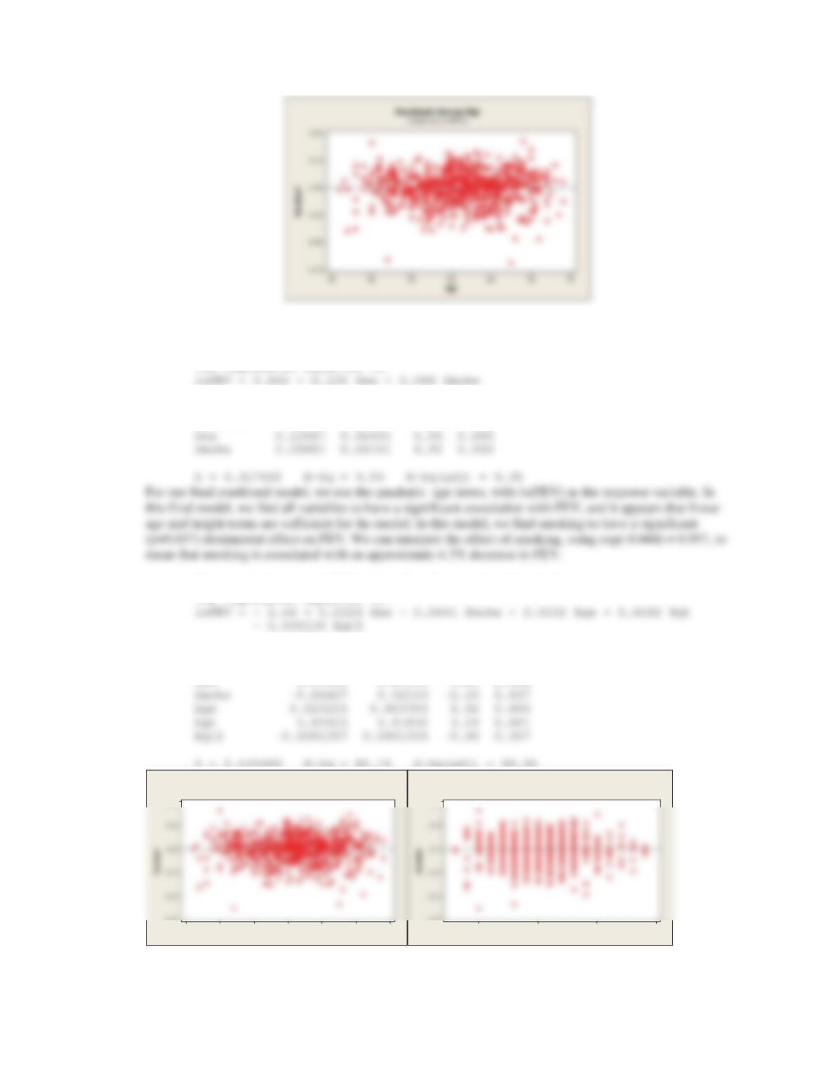
Taking what we have learned from the gender-specific analyses, we will use ln(FEV) as our response
variable, and investigate the need for quadratic age and height terms.
Regression Analysis: lnFEV versus Sex, Age, Age2
The regression equation is
Predictor Coef SE Coef T P
Constant -0.59220 0.06956 -8.51 0.000
2015105
Age
Residuals Versus Age
(response is lnFEV)
Regression Analysis: lnFEV versus Sex, Hgt, Hgt2
Predictor Coef SE Coef T P
Constant -2.9721 0.5646 -5.26 0.000
CHAPTER 11/REGRESSION AND CORRELATION METHODS 283
Again, we find a significant effect of smoking on FEV.
Regression Analysis: lnFEV versus Sex, Smoke
Predictor Coef SE Coef T P
Constant 0.82204 0.01852 44.39 0.000
Regression Analysis: lnFEV versus Sex, Smoke, Age, Hgt, Hgt2
The regression equation is
Predictor Coef SE Coef T P
Constant -2.4371 0.5521 -4.41 0.000
S = 0.145489 R-Sq = 81.1% R-Sq(adj) = 80.9%
75706560555045
0.50
-0.75
Hgt
Residuals Versus Hgt
(response is lnFEV)
2015105
0.50
-0.75
Age
Residuals Versus Age
(response is lnFEV)
284 CHAPTER 11/REGRESSION AND CORRELATION METHODS
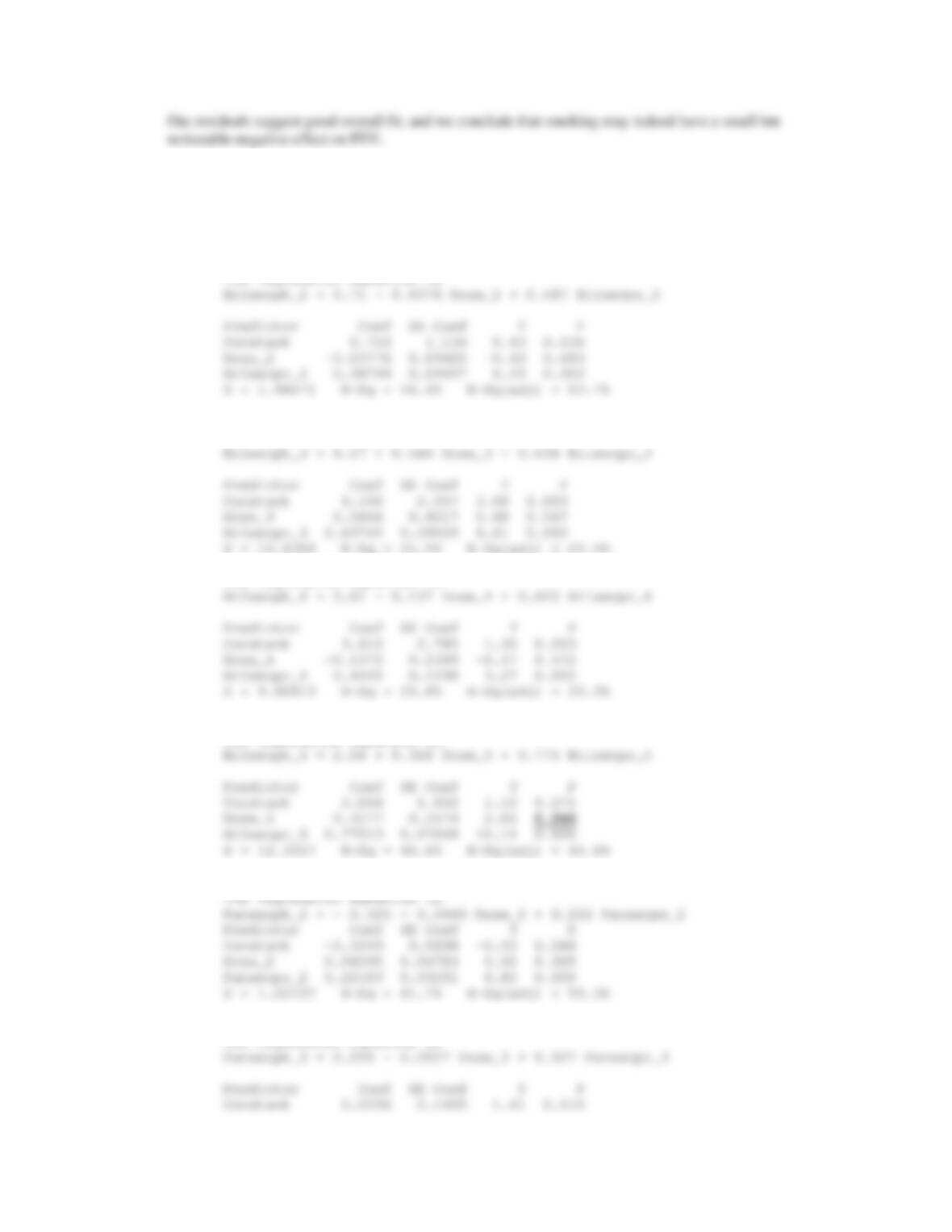
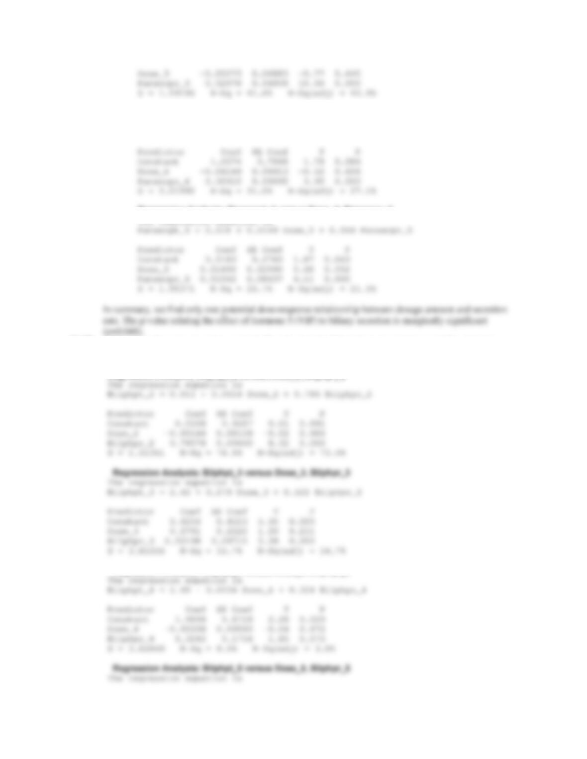
11.37 For this exercise, for each of the active hormones (2 – 5), we will regress the “post” values of biliary and
pancreatic secretion on both the dosage amount and the “pre” value. If there is a dose-response
relationship, then we expect to see a significant coefficient related with the dose covariate. Alternatively,
we could regress the difference = post-pre on the dosage amount. Results for biliary secretion are shown
first.
Regression Analysis: Bilsecpt_2 versus Dose_2, Bilsecpr_2
Regression Analysis: Bilsecpt_3 versus Dose_3, Bilsecpr_3
The regression equation is
S = 15.6369 R-Sq = 21.5% R-Sq(adj) = 20.5%
Regression Analysis: Bilsecpt_4 versus Dose_4, Bilsecpr_4
The regression equation is
Regression Analysis: Bilsecpt_5 versus Dose_5, Bilsecpr_5
The regression equation is
Regression Analysis: Pansecpt_2 versus Dose_2, Pansecpr_2
Regression Analysis: Pansecpt_3 versus Dose_3, Pansecpr_3
CHAPTER 11/REGRESSION AND CORRELATION METHODS 285
Regression Analysis: Pansecpt_4 versus Dose_4, Pansecpr_4
The regression equation is
Pansecpt_4 = 1.26 – 0.0415 Dose_4 + 0.359 Pansecpr_4
Regression Analysis: Pansecpt_5 versus Dose_5, Pansecpr_5
The regression equation is
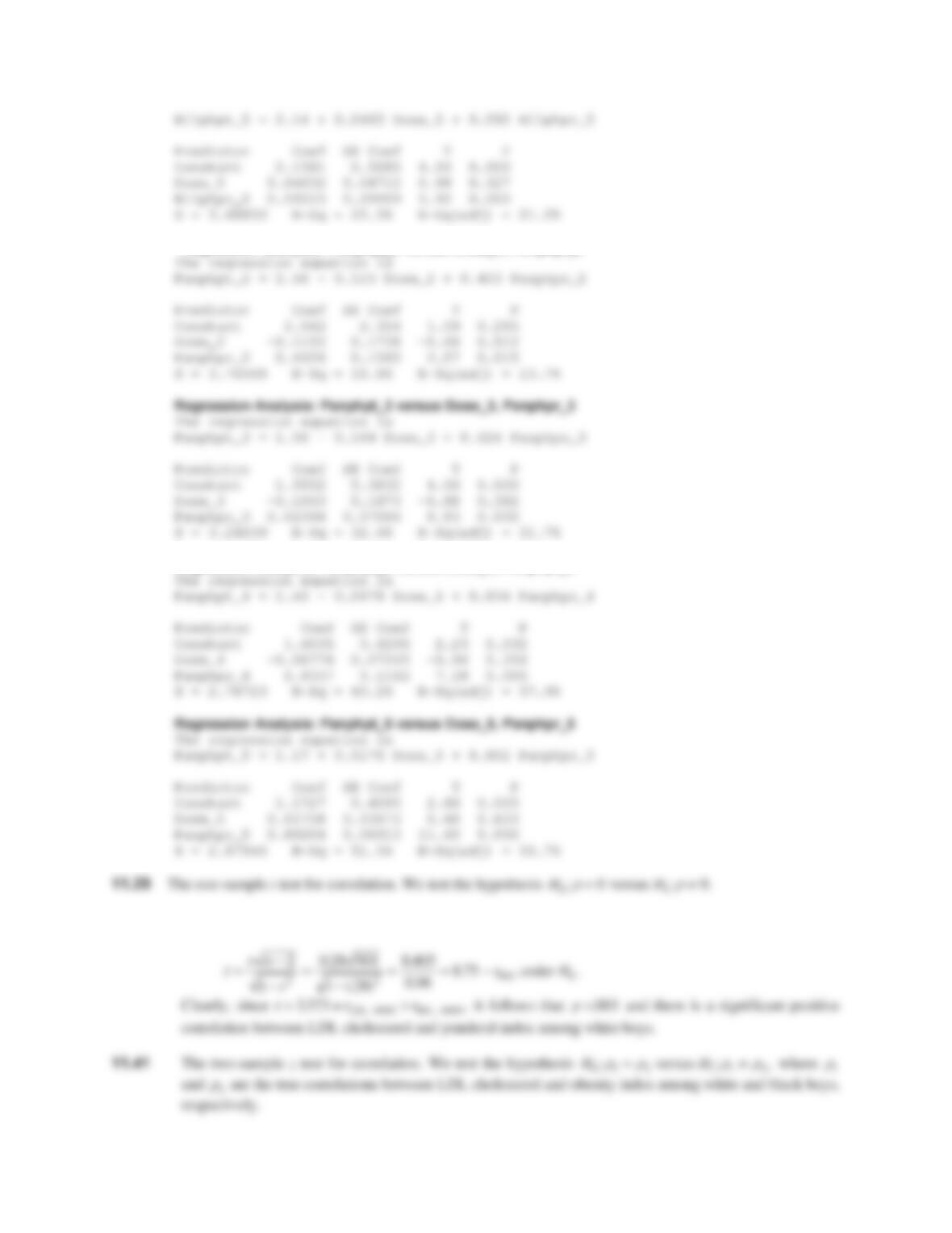
11.38 We repeat the same procedure as in 11.35, using “post” pH levels as our response variables this time.
We find no evidence of dose-response relationship with respect to pH levels.
Regression Analysis: Bilphpt_2 versus Dose_2, Bilphpr_2
Regression Analysis: Bilphpt_4 versus Dose_4, Bilphpr_4
286 CHAPTER 11/REGRESSION AND CORRELATION METHODS
Regression Analysis: Panphpt_2 versus Dose_2, Panphpr_2
Regression Analysis: Panphpt_4 versus Dose_4, Panphpr_4
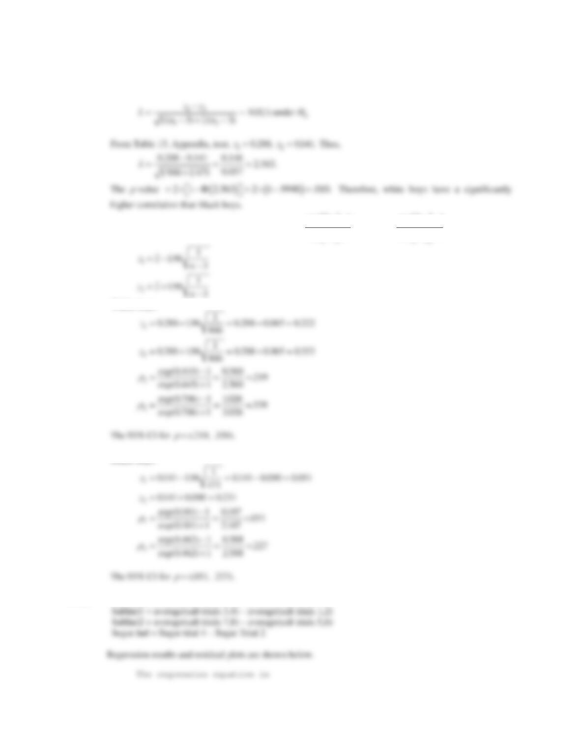
11.40 We have the test statistic
CHAPTER 11/REGRESSION AND CORRELATION METHODS 287
11.42 We have the test statistic
11.43 The 95% CI for is given by
U
1
,
U
2
,
where
U
1
exp 2z
1
1
exp 2z
1
1and
U
2
exp 2z
2
1
exp 2z
2
1
White boys
Black boys
11.44 The outcome variables we will use for this exercise are:
U