306 CHAPTER 11/REGRESSION AND CORRELATION METHODS
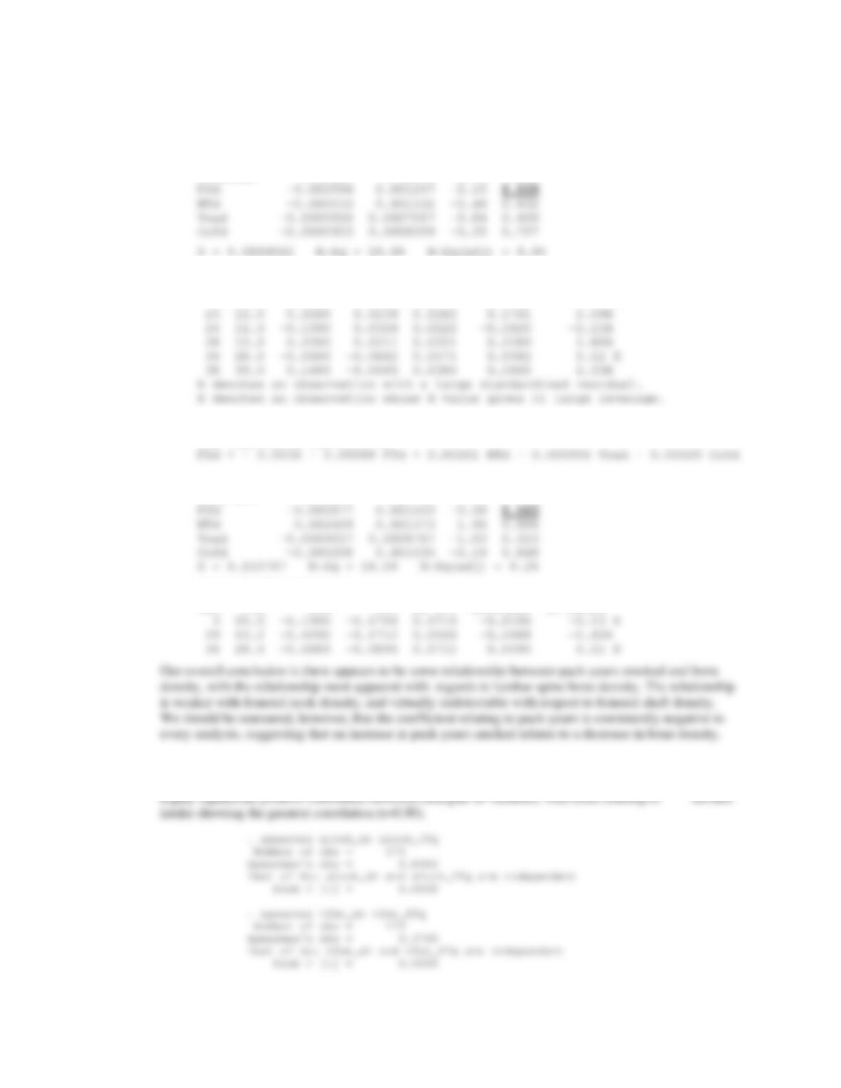
Regression Analysis: FNd versus PYd, WTd, Tead, Cofd
The regression equation is
FNd = 0.0532 – 0.00259 PYd – 0.00053 WTd – 0.000591 Tead – 0.000292 Cofd
Predictor Coef SE Coef T P
Constant 0.05323 0.02975 1.79 0.082
Unusual Observations
Obs PYd FNd Fit SE Fit Residual St Resid
3 20.5 0.0100 0.0268 0.0575 -0.0168 -0.25 X
Regression Analysis: FSd versus PYd, WTd, Tead, Cofd
The regression equation is
Predictor Coef SE Coef T P
Constant -0.00383 0.03705 -0.10 0.918
Unusual Observations
Obs PYd FSd Fit SE Fit Residual St Resid
11.72-11.75
We can use STATA to calculate the rank correlation for each of these pairs of observations. We find
CHAPTER 11/REGRESSION AND CORRELATION METHODS 307
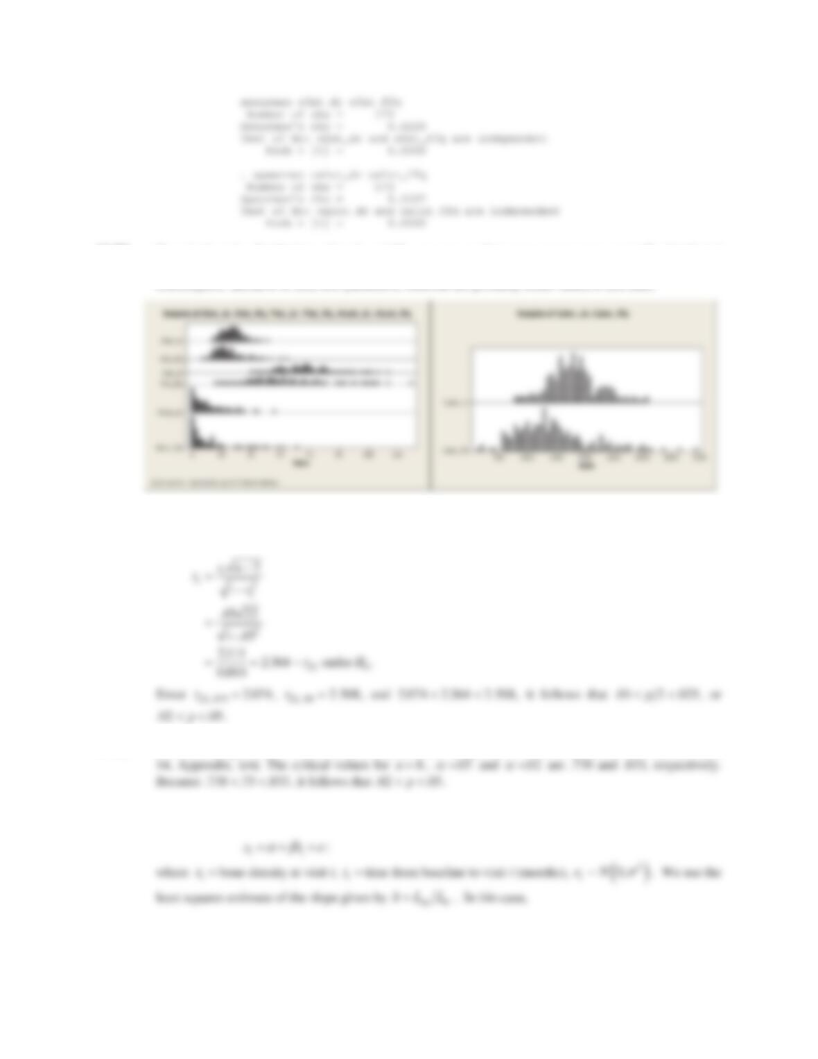
11.76 If we look at the distributions of each variable, we can see that some appear more normally distributed
than others. Many of the distributions appear be skewed to the right, especially those relating to alcohol
consumption. Because of this, non-parametric methods are probably better suited to this data.
11.77 We wish to test the hypothesis : vs : , where is the true rank correlation. We
use the test statistic
11.78 Since the sample size is , we must use the small sample test for rank correlation. We refer to Table
D
D
11.79 We use the linear regression model
H0
U
s 0H1
U
sz0
U
s
10
308 CHAPTER 11/REGRESSION AND CORRELATION METHODS
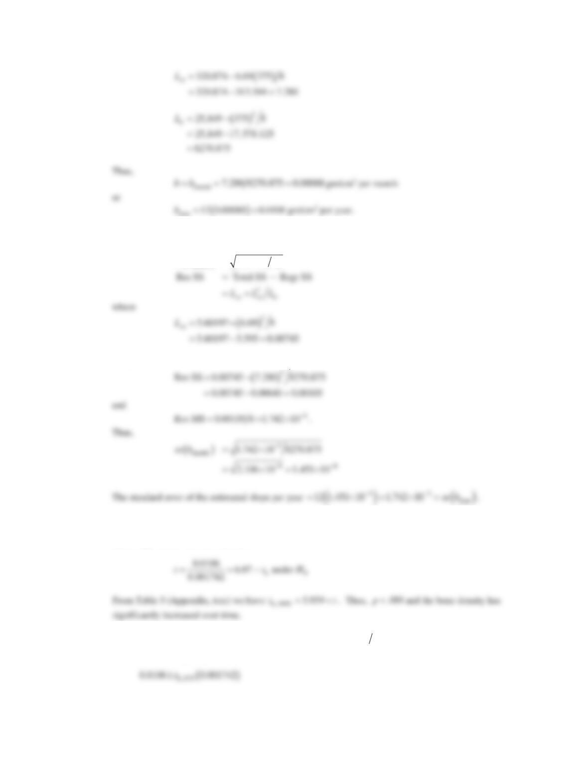
To obtain the standard error,
month
Res MS
tt
se b L
Thus,
11.80 We wish to test the hypothesis 01
:0vs.:0HH
E
E
z
. We will use the one sample t-test for ordinary
linear regression. The test statistic is:
11.81 The normal rate of change per year from age 40 to age 80 is 0.15 40 0.00375 gm/cm2 per year 0
E
. A 95% CI for year
E
is given by
CHAPTER 11/REGRESSION AND CORRELATION METHODS 309
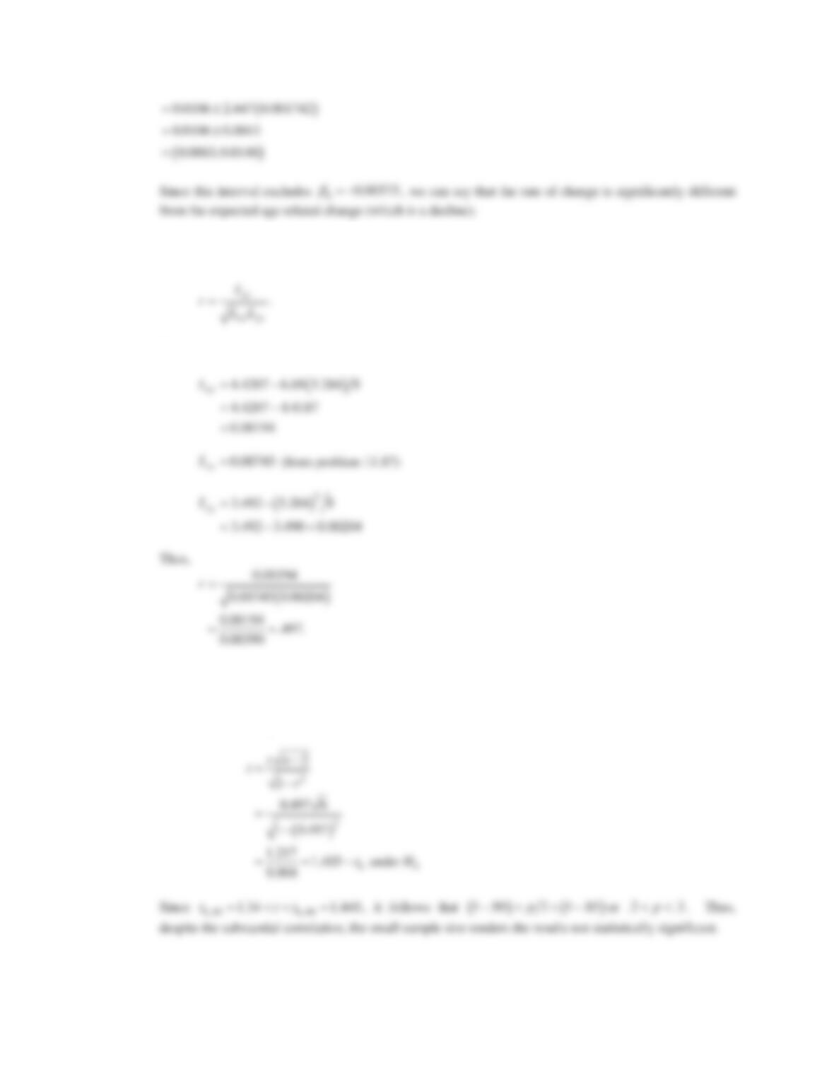
11.82 A measure of association relating bone density of the lumbar spine vs. bone density of the femoral neck
is the correlation coefficient (r) given by
We have
11.83 We wish to test the hypothesis 01
:0vs.:0HH
U
U
z
where
U
is the underlying correlation between
bone density of the lumbar spine and bone density of the femoral neck.
We use the one sample t test for correlation. The test statistic is
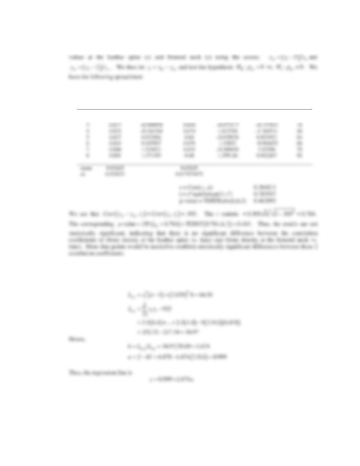
310 CHAPTER 11/REGRESSION AND CORRELATION METHODS
11.84 We wish to test the hypothesis 0:
x
tyt
H
U
U
. For this purpose, we first standardize the bone density
Spreadsheet for Solution to Problem 11.80
i i
x
s
i
x
i
y
s
i
y
s
isii
x
yz
i
t
1 0.797 –1.202842 0.643 –0.758249 –0.444593 0
2 0.806 –0.927031 0.638 –1.044381 0.11735 8
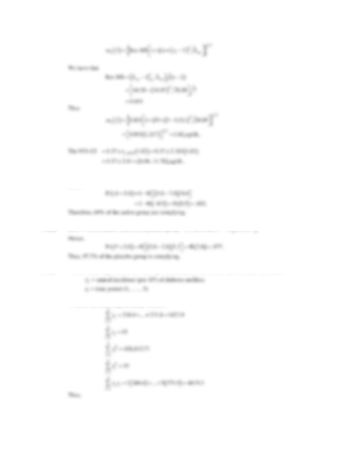
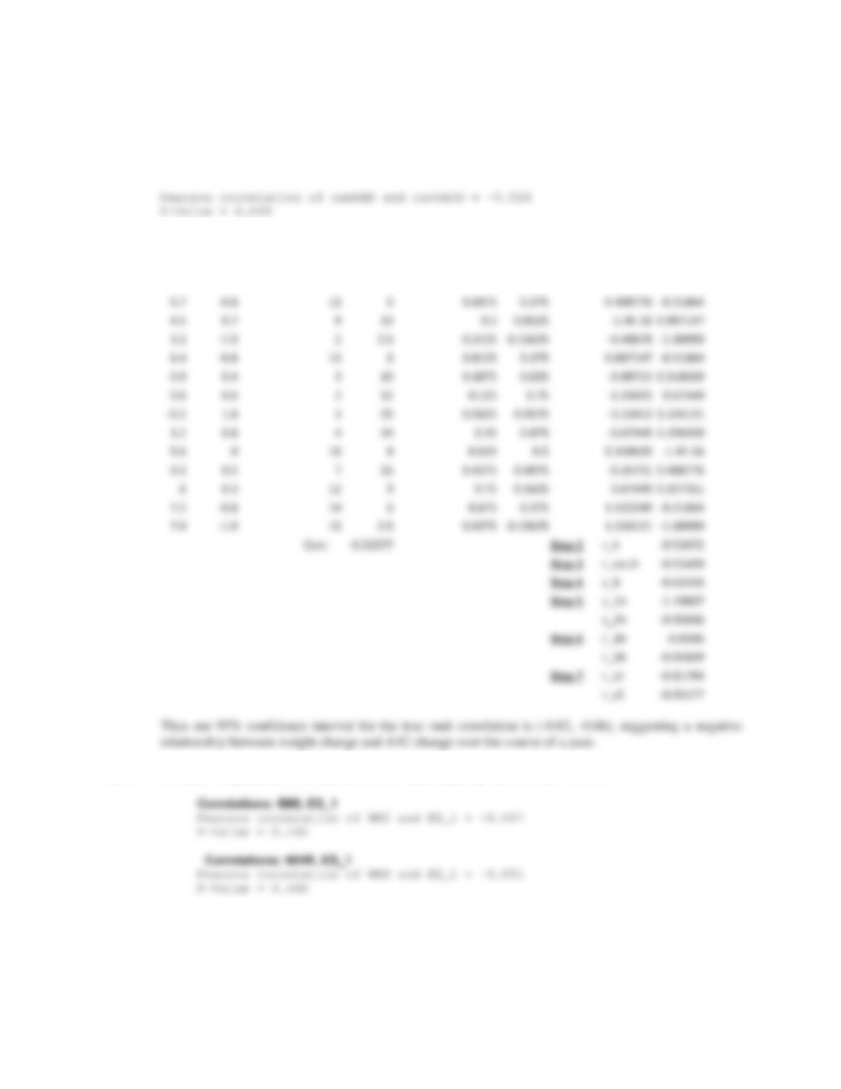
11.85 We use the method of least squares, where y = serum lutein 2003, x = serum lutein 1999. We have
2
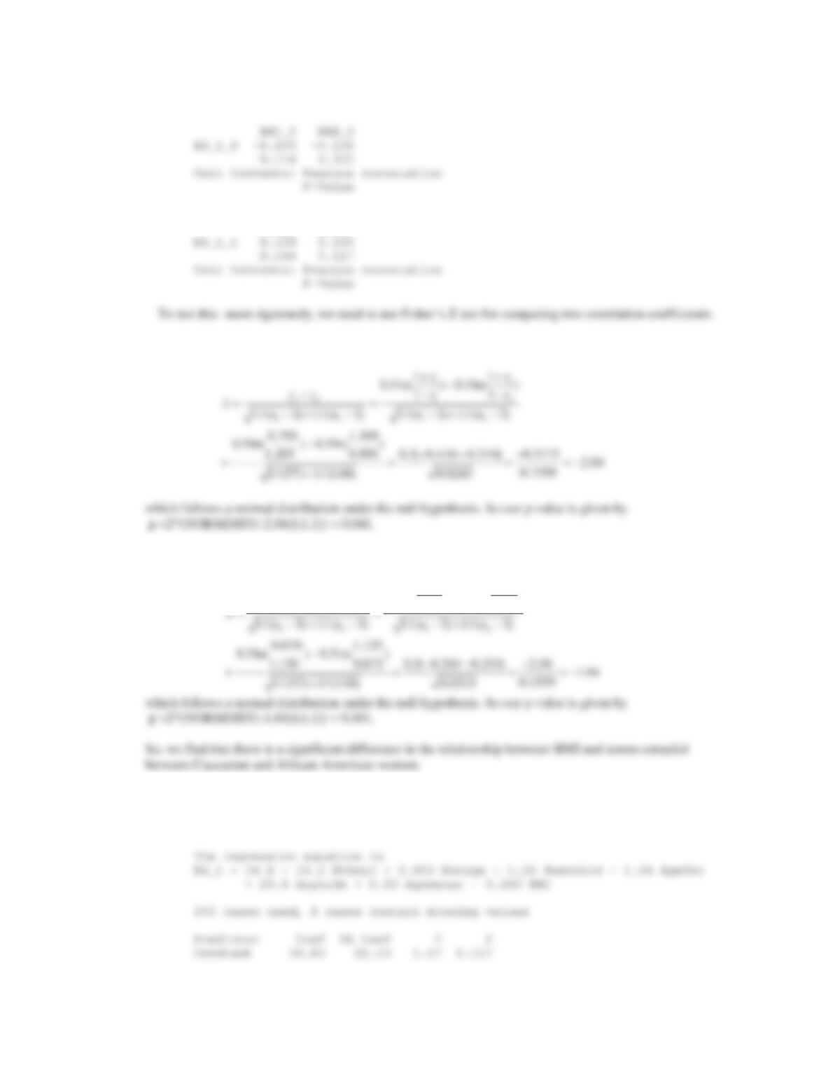
2
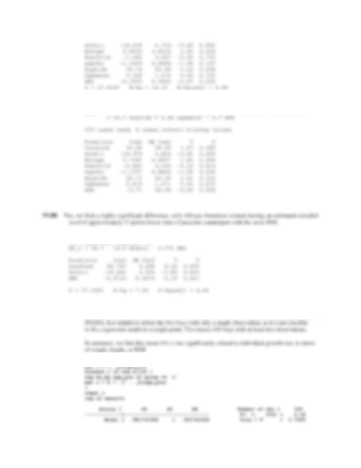
1 1.616 8 20.89
xx x
Lsn
11.86 The predicted serum lutein value based on the 2003 assay is
ˆ0.999 1.674 5 9.37 g/dLy
P
. The
standard error of this estimate is
s
CHAPTER 11/REGRESSION AND CORRELATION METHODS 311
11.87 Let A = serum lutein value in the active group. We have that
2
7.0, 4.0AN.
Hence,
11.88 Let P = serum lutein value in the placebo group. We have that
2
2.0, 1.5PN.
11.89 We use linear regression to solve this problem, based on the model iii
yxe
D
E
, where
We have the following summary statistics:
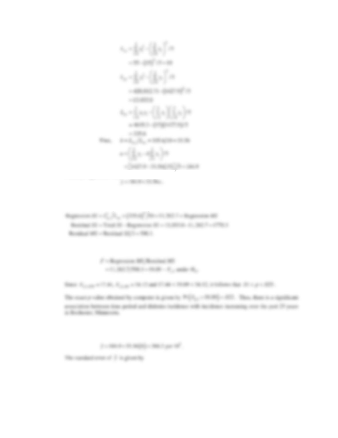
312 CHAPTER 11/REGRESSION AND CORRELATION METHODS
¬¼
Thus, the regression line is
11.90 We wish to test the hypothesis 01
:0vs.:0HH
E
E
z
. We will use the F test for simple linear
regression. We have that
The F statistic is given by
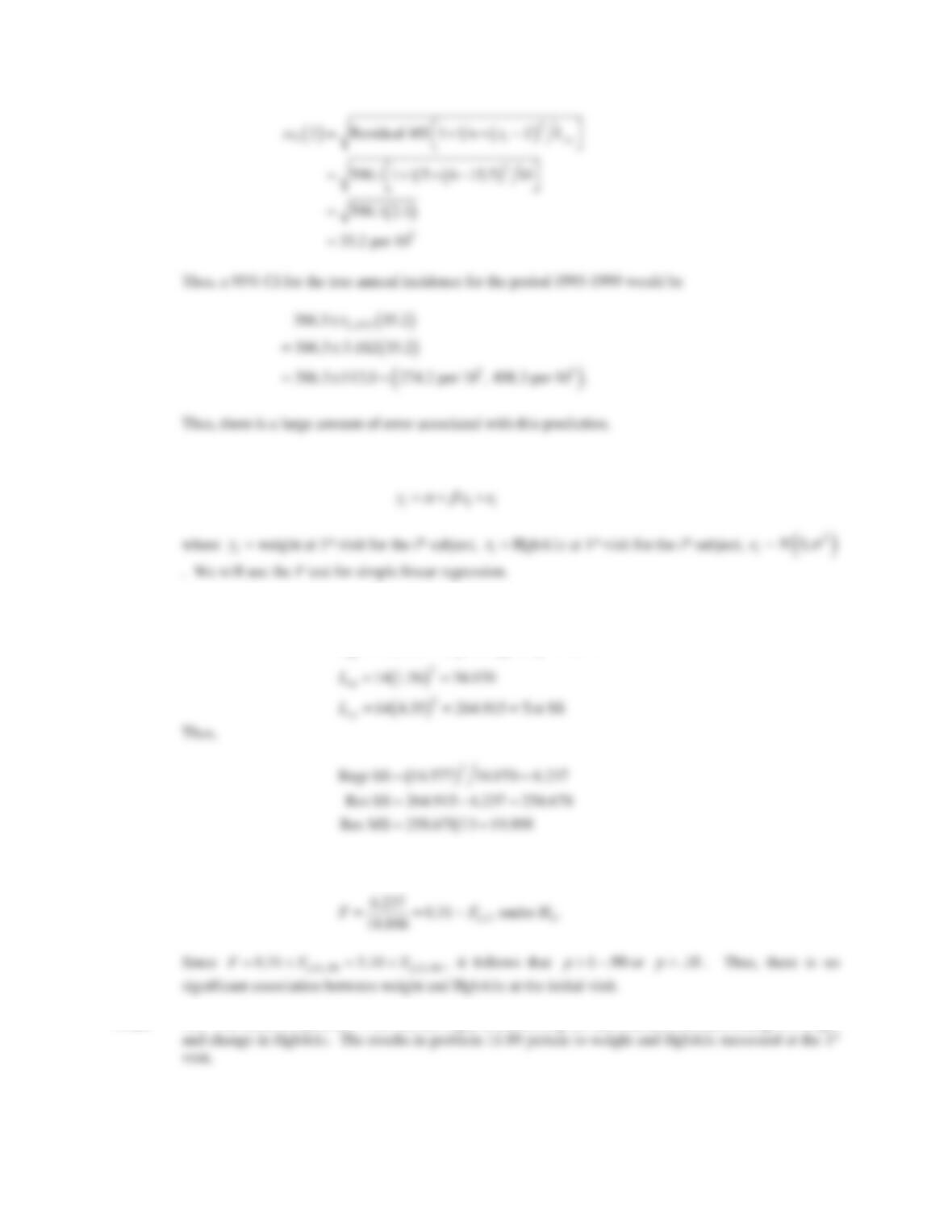
11.91 The time period 1995-1999 would correspond to a time period score of 6. Thus, from the regression
equation in Problem 11.85 the predicted incidence would be
CHAPTER 11/REGRESSION AND CORRELATION METHODS 313
11.92 We will use the linear regression model.
11.93 We have that
4722.09 15 37.63 8.34 14.577
xy
L
Thus, the test statistic is
11.94 No. The results in problem 11.89 do not imply a relationship (or lack thereof) between change in weight
314 CHAPTER 11/REGRESSION AND CORRELATION METHODS
11.95 For this analysis, we will use MINITAB to convert the original data to ranked data, as well as to estimate
the rank correlation and p-value. Then we use Excel to derive the 95% confidence interval for the true
underlying rank correlation. For sample Excel code, see 11.67
Correlations: rankWD, rankA1D
WgtDA1cDrankWDrankA1DWDͲPA1DͲPWDͲProbA1DͲProb
5Ͳ1.59 4 0.5625 0.25 0.157311Ͳ0.67449
3.8Ͳ2.16 1 0.375 0.0625 Ͳ0.31864Ͳ1.53412
11.96 We find no significant association between either adiposity measure and estradiol.
11.97 While the correlations are not significant within either ethnic group, we do note that we find slight
negative correlations between adiposity and estradiol in Caucasian women, and slight positive
correlations in African-American women.
CHAPTER 11/REGRESSION AND CORRELATION METHODS 315
Correlations: BMI_0, WHR_0, ES_1_0
Correlations: BMI_1, WHR_1, ES_1_1
BMI_1 WHR_1
For the relationship between Estradiol and BMI, we have
For the relationship between Estradiol and WHR, we have
12
12 1 2
11
0.5ln( ) 0.5ln( )
11
rr
zz r r
11.98 To address this question, we can create a regression model containing each of the six listed risk factors, in
addition to each of our adiposity measures. We show the results of both regressions below, and find no
significant relationship between either adiposity with estradiol, after controlling for other risk factors.
316 CHAPTER 11/REGRESSION AND CORRELATION METHODS
Regression Analysis: ES_1 versus Ethnic, Entage, …
The regression equation is
ES_1 = 30.7 – 17.0 Ethnic + 0.758 Entage – 0.84 Numchild – 1.14 Agefbo
S = 27.8512 R-Sq = 9.9% R-Sq(adj) = 6.7%
Regression Analysis: ES_1 versus Ethnic, BMI
The regression equation is
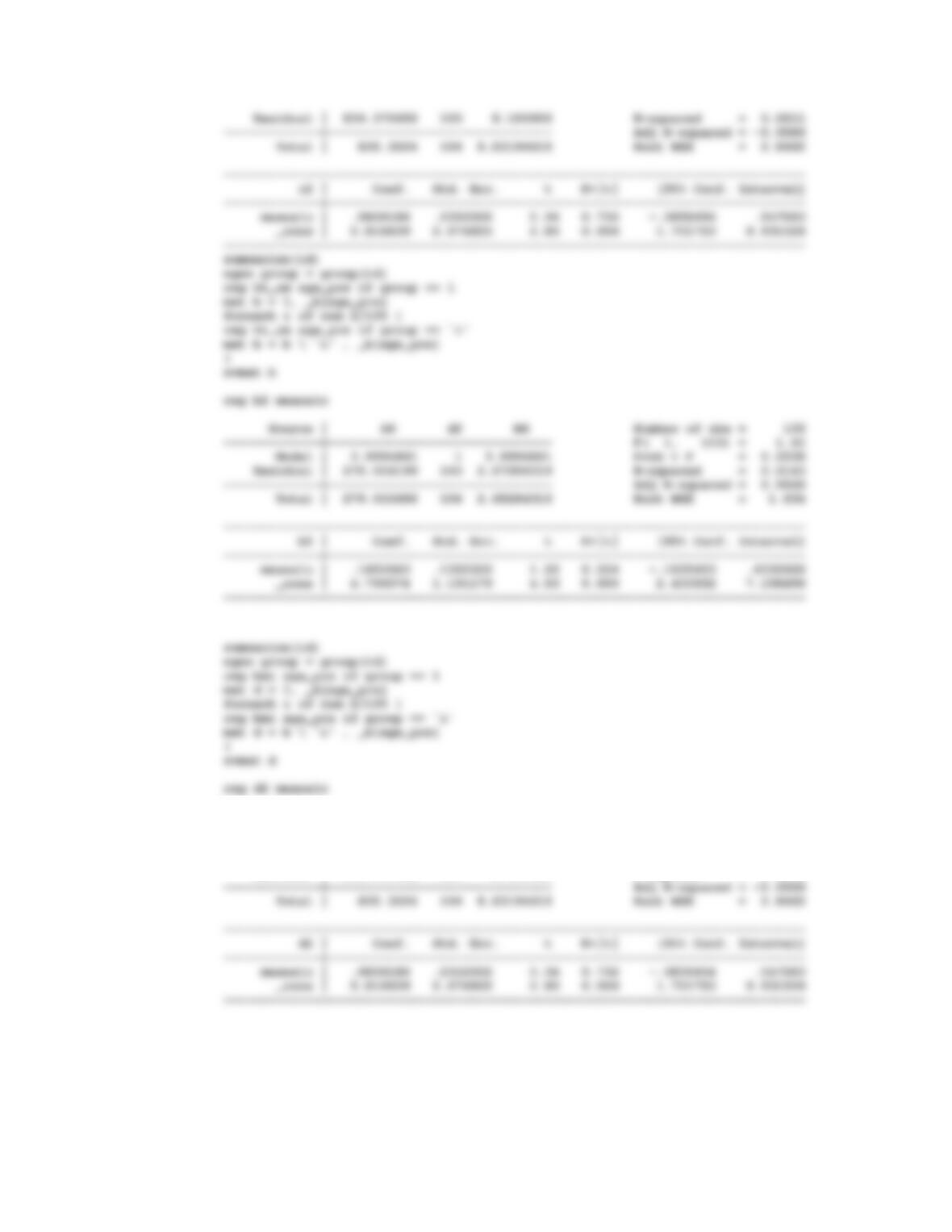
11.100-11.102 For each of these problems, we need to run a regression model and store the appropriate regression
coefficient for each boy. Below, we show an example of code that will perform these operations in
reg wt_kg age_yrs if group == 1
CHAPTER 11/REGRESSION AND CORRELATION METHODS 317
Source | SS df MS Number of obs = 105
————-+—————————— F( 1, 103) = 0.12
Model | .951741928 1 .951741928 Prob > F = 0.7325
Residual | 834.370658 103 8.100686 R-squared = 0.0011
11.103 We will use the linear regression model.
318 CHAPTER 11/REGRESSION AND CORRELATION METHODS
11.104 We have the following summary statistics:
1
i
Thus,
[82.852 0.0347 66.99 ] / 11 7.743
Thus, the regression line is
The F statistic is given by
CHAPTER 11/REGRESSION AND CORRELATION METHODS 319
1,9,.95 1,9,.975
11.105 The intercept of 7.743 means that we estimate the patients ln(visual area) at baseline to be 7.743, which
11.106 Using the regression model, we estimate ˆ7.743 0.0347(20) 7.05y
The prediction interval is given by
11.109 We can test whether or not there is a significant relationship between the two variables by testing
11.110 The residual variance was calculated above as
320 CHAPTER 11/REGRESSION AND CORRELATION METHODS
22
2
/0.744 / 1.2
xy xx
LL
11.112 We use the one-sample t-test for correlation. We have the test statistic:
11.113 We use the Fisher z method to obtain a 95% CI for ȡ. We have:
z 0.5 ln 1 + 0.313
1 – 0.313
§
©
¨
·
¹
¸ 0.324.
11.115 The regression coefficient given in Table 11.37 is -0.0875 and refers to the expected difference in
11.118 Our data is r=0.448, n=12. To test for significant correlation, we will use Eq. 11.20, and our t-statistic is
(10)
CHAPTER 11/REGRESSION AND CORRELATION METHODS 321
11.119 To generate a 95% confidence interval, we must first take the Fisher transformation of our sample
correlation.
11.120 The rank data is shown at right.
FFQDRFFQͲrankDRͲrank
707.52.5
70.57.55.5
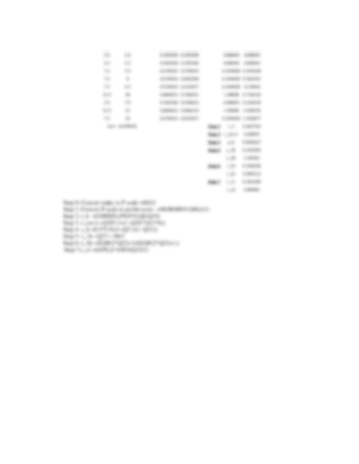
11.121 To calculate the 95% confidence interval for the Spearman rank correlation, we need to follow the
procedure described in Eq. 11.40. The rank data and Excel worksheet are shown below, along with
sample coding. The final CI is (0.182, 0.897).
322 CHAPTER 11/REGRESSION AND CORRELATION METHODS
2.52.50.192308 0.192308 Ͳ0.86942 Ͳ0.86942