CHAPTER 10/HYPOTHESIS TESTING: CATEGORICAL DATA 253
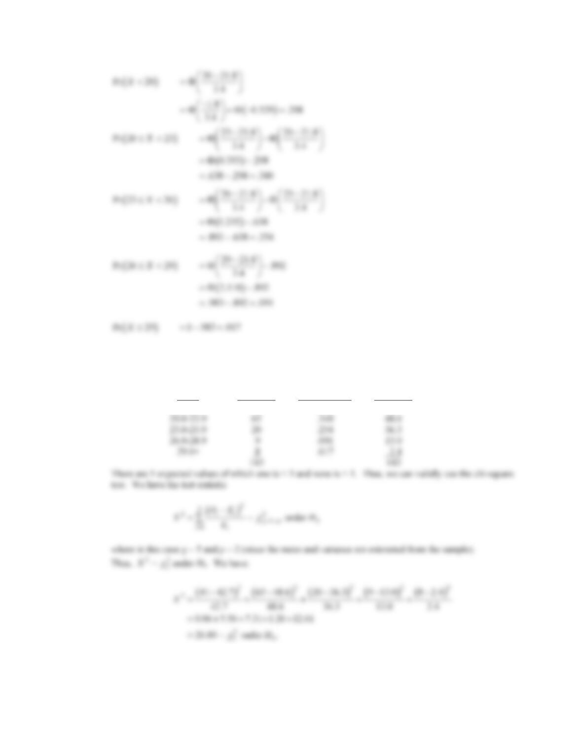
To compute the expected count in each group we multiply the probabilities by the grand total (143) as
follows:
BMI
group
Observed
frequency
Probability
Under a
normal model
Expected
frequency
19.9d41 .298 42.7
254 CHAPTER 10/HYPOTHESIS TESTING: CATEGORICAL DAT
A
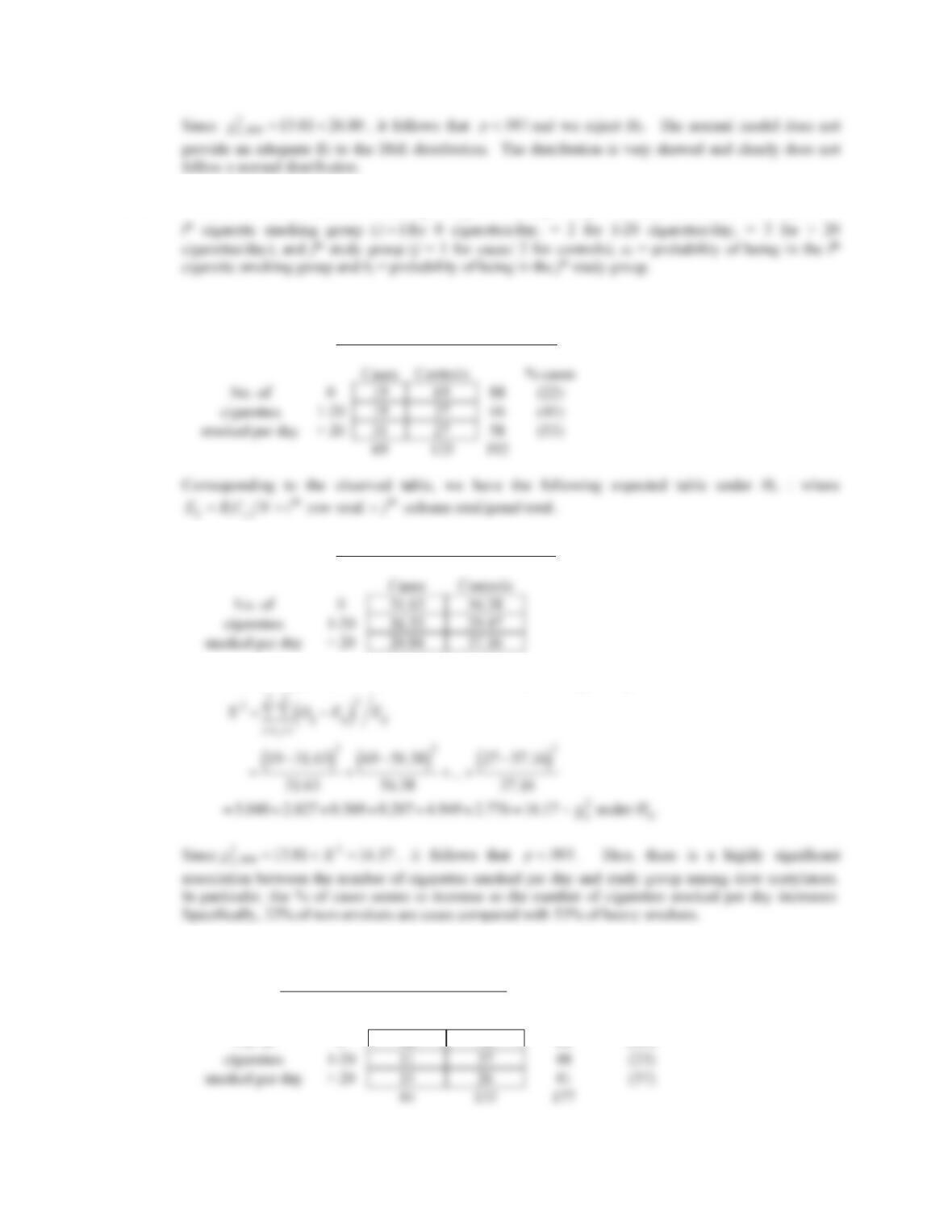
10.101 We wish to test the hypothesis 01
:vs.:
ij ij ij ij
H
pab Hpab z
where pij = probability of being in the
We have the following observed table:
Observed Table – Slow Acetylators
Expected Table – Slow Acetylators
We use the chi-square test for RCutables. The test statistic is given by:
10.102 We use a similar approach as in problem 10.102. We have the following observed and expected tables:
Observed Table – Rapid Acetylators
Cases Controls % cases
No. of 0 18 70 88 (20)
CHAPTER 10/HYPOTHESIS TESTING: CATEGORICAL DATA 255
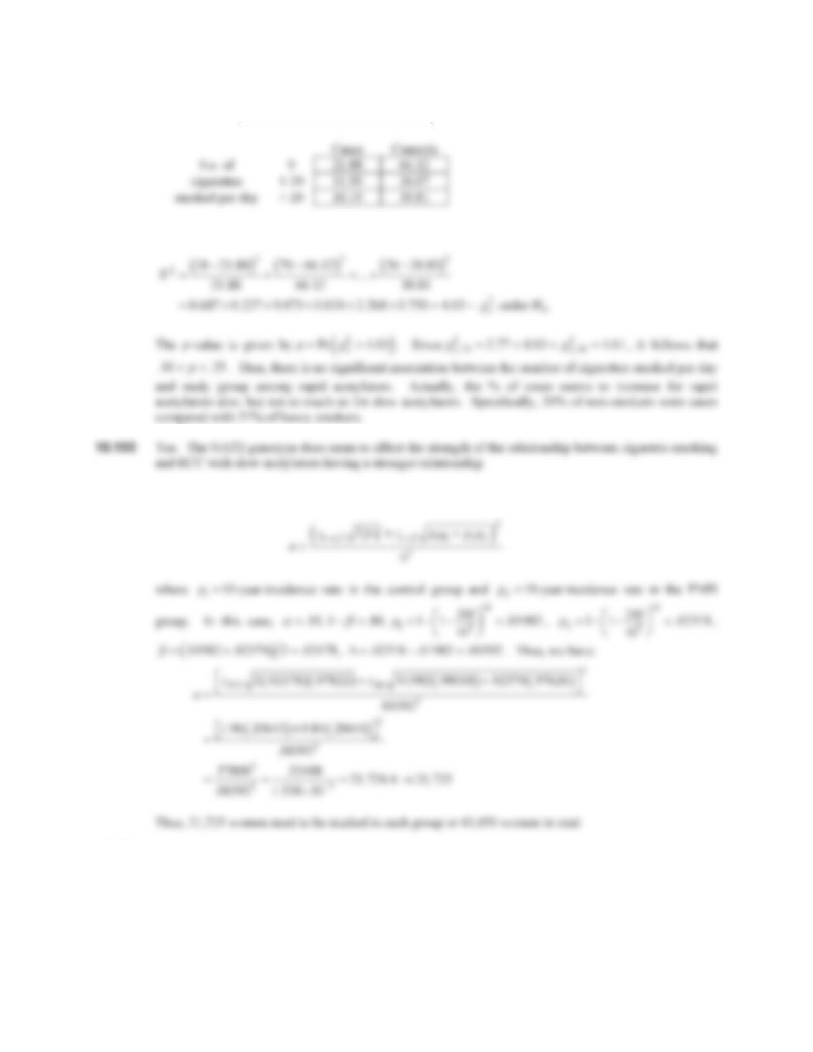
Expected Table – Rapid Acetylators
The chi-square statistic is given by
10.104 We use the sample size formula
10.105 The power of the study is given by
256 CHAPTER 10/HYPOTHESIS TESTING: CATEGORICAL DAT
A
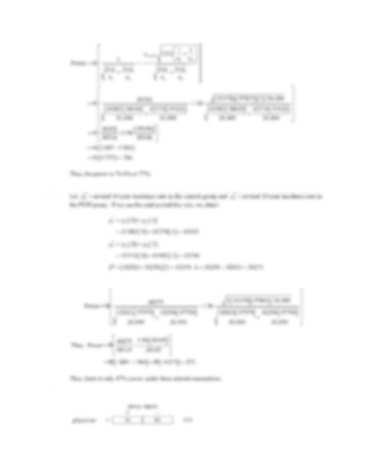
10.106 The incidence rate of breast cancer will change in each treatment group due to these altered assumptions.
Thus, the revised power is given by
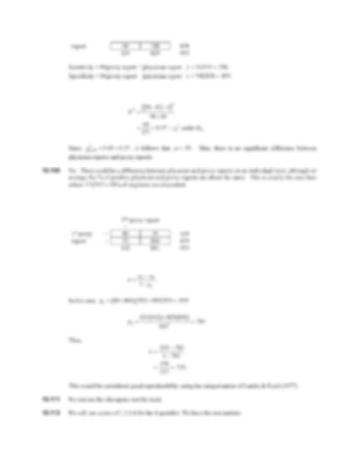
10.107 We have the following 22utable
CHAPTER 10/HYPOTHESIS TESTING: CATEGORICAL DATA 257
10.108 We will use McNemar’s test for correlated proportions. We have the test statistic
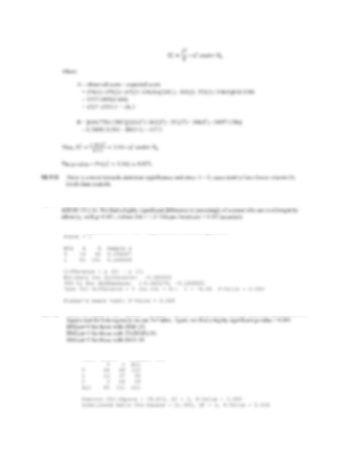
10.110 We have the following 22utable
We will compute the Kappa coefficient as an index of reproducibility of the proxy reports. We have
258 CHAPTER 10/HYPOTHESIS TESTING: CATEGORICAL DAT
A
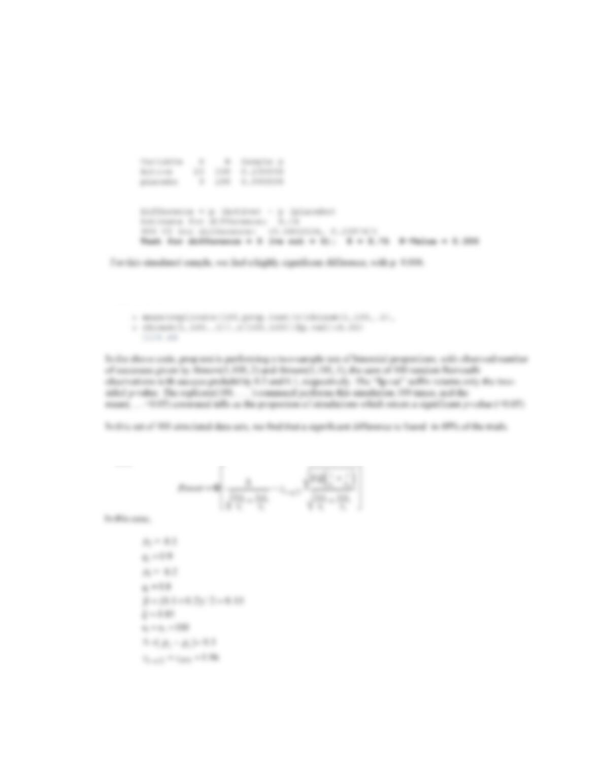
10.114 We perform a two-sample test of binomial proportions, after creating a new variable “overweight” =
Test and CI for Two Proportions: Overweight, Eth
10.115 Here, we create a new variable “BMIcat”= if(‘BMI'<25,0,if(‘BMI’>30,2,1)), and then perform a Chi-
Tabulated statistics: BMIcat, Eth
Rows: BMIcat Columns: Eth
CHAPTER 10/HYPOTHESIS TESTING: CATEGORICAL DATA 259
10.116 In MINITAB, we generate 100 rows of random data following a Bernoulli(p=0.2) distribution, and store
in one column, then generate 100 rows of data coming from a Bernoulli(p=0.1) distribution, and store in
a second column. Then we use the “2 proportions” option to compare the two columns.
Test and CI for Two Proportions: Active, placebo
Event = 1
10.117 This problem is easiest to address in a programming language like R: The following code will give the
desired answer:
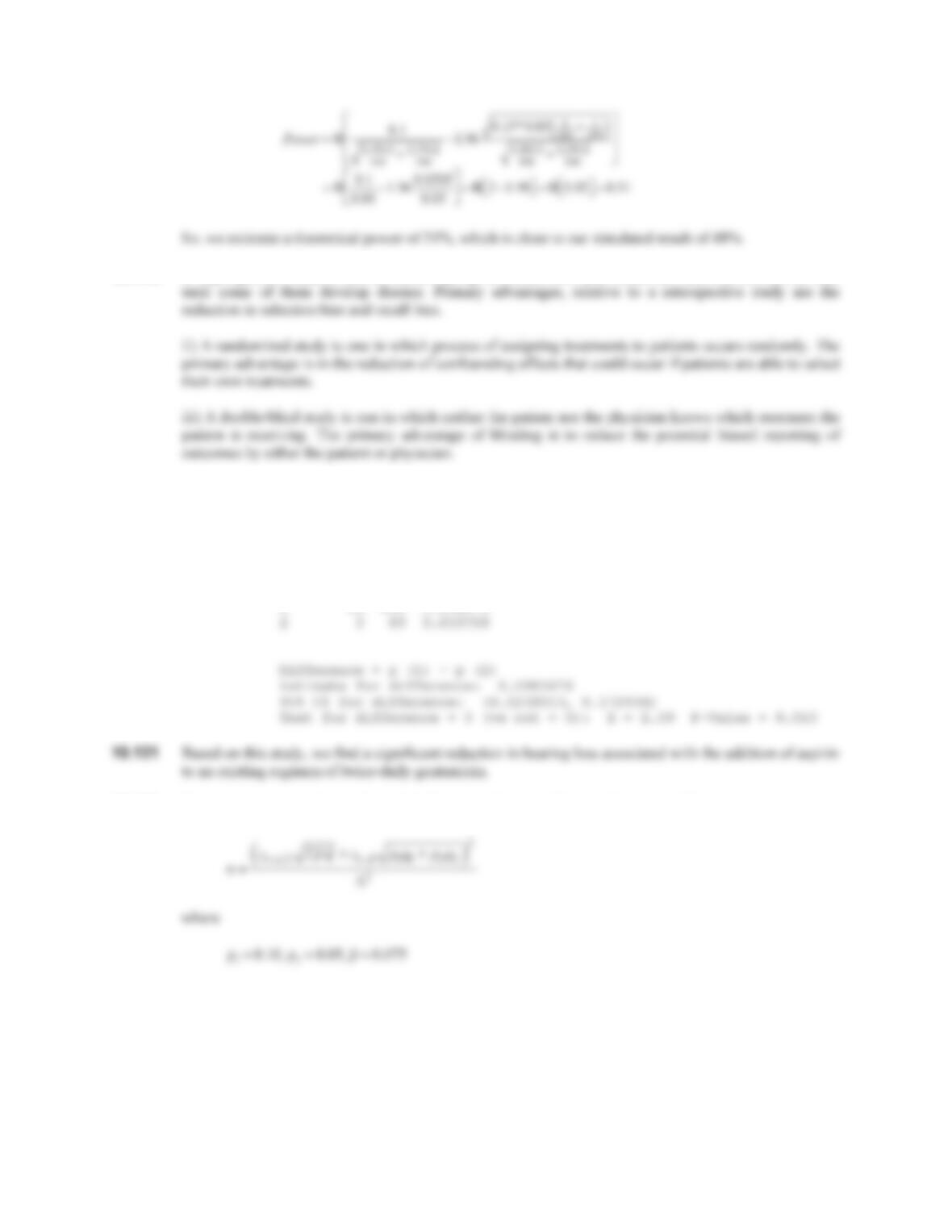
10.118 We use the power formula for comparing two binomial proportions (see Equation 10.14 in Chapter 10,
text)
Therefore, the power is given by:
260 CHAPTER 10/HYPOTHESIS TESTING: CATEGORICAL DAT
A
10.119 i) A prospective study is one in which a group of disease-free individuals are followed forward in time
10.120 We will use a two-sample test for binomial proportions. We show output below from MINITAB, which
reports a p-value of 0.01. However, this method does not use a continuity correction. The correct p-value,
with continuity correction, is p=0.03.
Test and CI for Two Proportions
Sample X N Sample p
1 14 106 0.132075
10.122 First we use the sample size formula in Equation 10.14 (in Chapter 10, text) as follows
CHAPTER 10/HYPOTHESIS TESTING: CATEGORICAL DATA 261
Thus, with perfect compliance, we would need to enroll 581 persons in each group to achieve a 90%
power.
10.124 P(True + | Test +) = P(True+, Test+)/P(Test+)
10.125 We need to use the exact version of McNemar’s test, because the number of discordant pairs is
10.126 The number of matched pairs is
262 CHAPTER 10/HYPOTHESIS TESTING: CATEGORICAL DAT
A
10.127 A nominal categorical variable represents one in which different data values represent different
10.128 Since we are treating ocular discomfort as a nominal variable, we use the Chi-Square test for
10.129 Treating ocular discomfort as an ordinal variable, we want to use the Chi–Square test for trend. We can
use the ocular discomfort scores (2, 3, 4) as the score values.
We have the test statistic , where
10.130 To test whether there is an association between the salt taste response and DBP quintile, we test the null
10.131 The expected number of infants in DBP quintile 2 with preferential salt test response under the null
hypothesis is
XAB
1
22
CHAPTER 10/HYPOTHESIS TESTING: CATEGORICAL DATA 263
10.132 We can use the chi-square test for trend. We have the test statistic , where
10.133 We can also perform the whole test using R
10.137 Let
10.138 Our observed, expected, and
X
2
(OE)
2
/E
values are shown below
Observed Expected Chi-Sq values
Event No Event N Event
No
Event Event No Event
Aspirin 20 537 557 12.8046 544.1954 4.04 0.10
XAB
1
22
264 CHAPTER 10/HYPOTHESIS TESTING: CATEGORICAL DAT
A
10.140 We will use “x” to denote the number of cases in each risk score group, and we will use the given risk
scores (1, 2 . . . 6) as our S values.
10.141 P(AMD+|Score=1) = P(Score=1|AMD+)*P(AMD+)/P(Score=1)
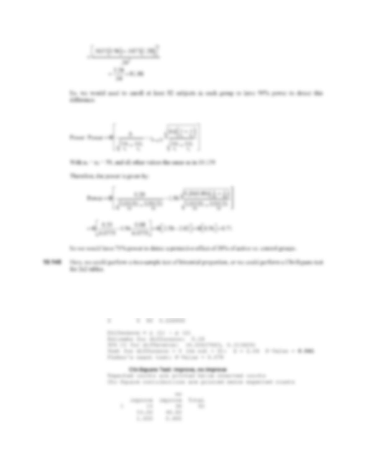
10.143 We use the sample size formula in Equation 10.14 (in Chapter 10, text) as follows
ScoreCasesControlsTotalx*Sn*Sn*S2
13111431414
CHAPTER 10/HYPOTHESIS TESTING: CATEGORICAL DATA 265
10.144 We will use the following power formula
10.146 We show both results below using MINITAB.
Test and CI for Two Proportions
Sample X N Sample p
1 14 50 0.280000
266 CHAPTER 10/HYPOTHESIS TESTING: CATEGORICAL DAT
A
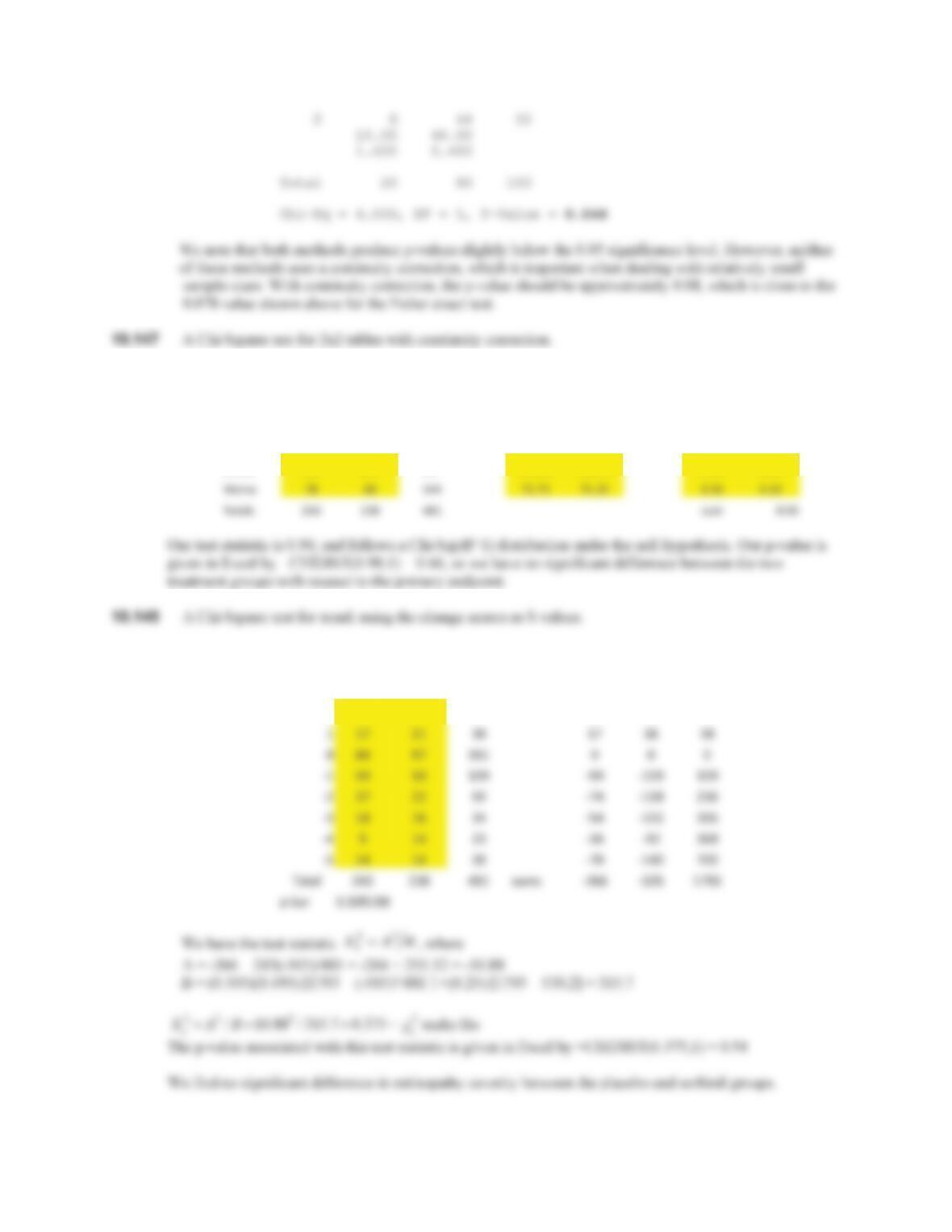
10.148 After collapsing the original 2×8 table into a 2×2 table, our observed, expected, and
X
2
(| OE|0.5)
2
/E
values are shown below
ObservedExpectedChiͲSquareValue
PlaceboSorbinilTotalsPlaceboSorbinilPlaceboSorbinil
Better165172337170.25166.750.130.14
10.150 Data is shown below, with x representing the number of patients in the placebo group for a given change
score.
ChangePlaceboSorbinilTotalx*Sn*Sn*S2
2549101836
CHAPTER 10/HYPOTHESIS TESTING: CATEGORICAL DATA 267
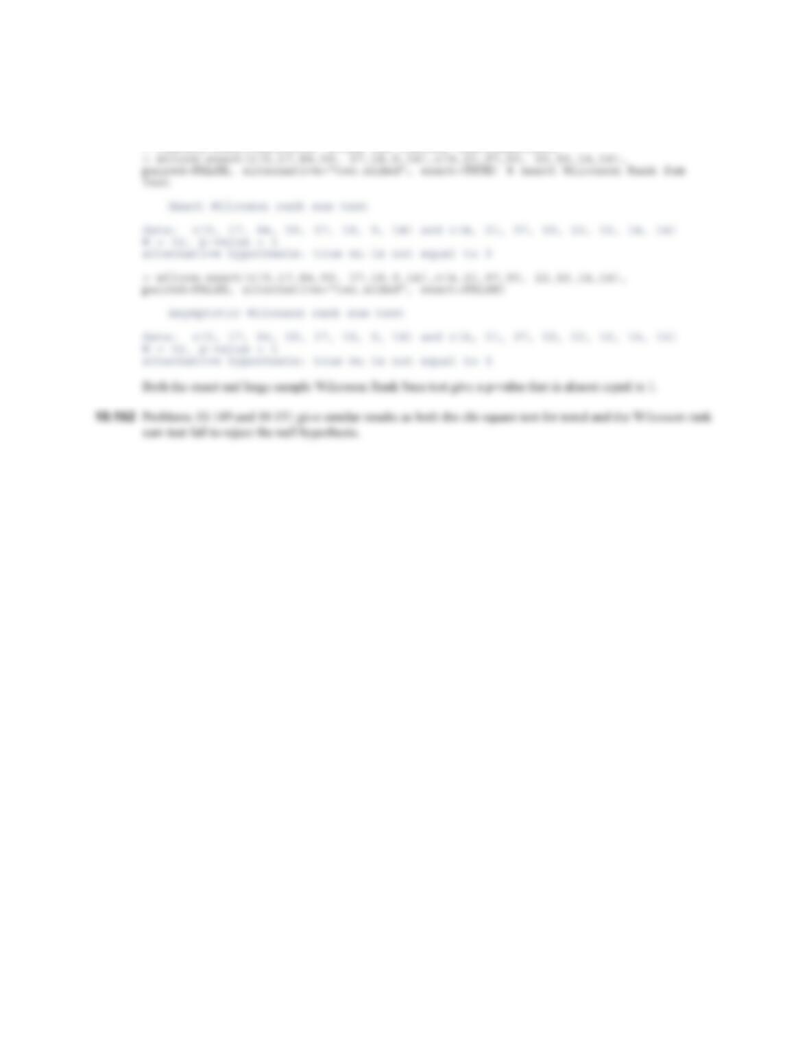
10.151 We use the command “wilcox.exact” from the library exactRankTests to run the Wilcoxon rank sum test
with ties
> library(exactRankTests) #load the library exactRankTests