CHAPTER 10: Standard Costing and Variance Analysis
E 10-58 ↓ links ↓
change here, please ↓
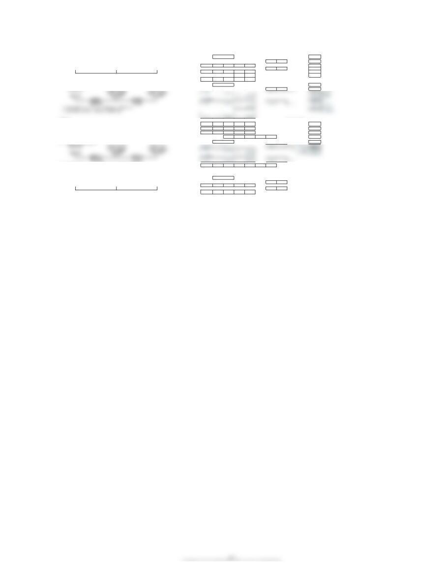
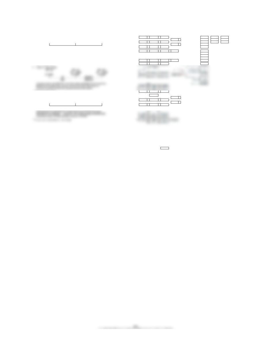
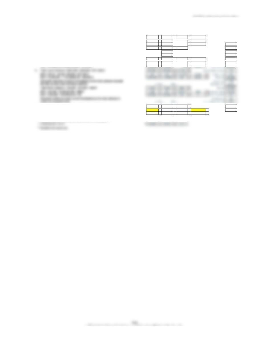
1. Variable overhead analysis: Actual VOH: 4Lbs. of RM reqd.
1,170 U Spending 36 DLH
0.70 × 158,900 = 111,230 18.00 wage rate
Applied VOH: (210) F Efficiency 2Hrs. reqd.
0.70 × 79,600 × 2 80,000 Practical volume
Standard hours: = 111,440 11.20 Direct materials
*Standard Hours = 2 hours × 79,600 units = 159,200 hours 2 × 79,600 = 159,200
2. Fixed overhead analysis: Actual FOH: 2.80 Lbs. rate
Budgeted FOH: (1,000) F Spending 18.10 Act. Wage rate
5.20 × 80,000 × 2 831,000 Fixed OH
Applied FOH: 158,900 DLH
*Practical Volume in Hours = 2 hours × 80,000 units = 160,000 hours = 827,840 5.20 Fixed O/H rate
$1,000 F
Spending
Budgeted FOH
$5.20 × 160,000*
$832,000
Actual FOH
$831,000
$4,160 U
Applied FOH
$5.20 × 159,200**
$827,840
E 10-59
change here, please ↓
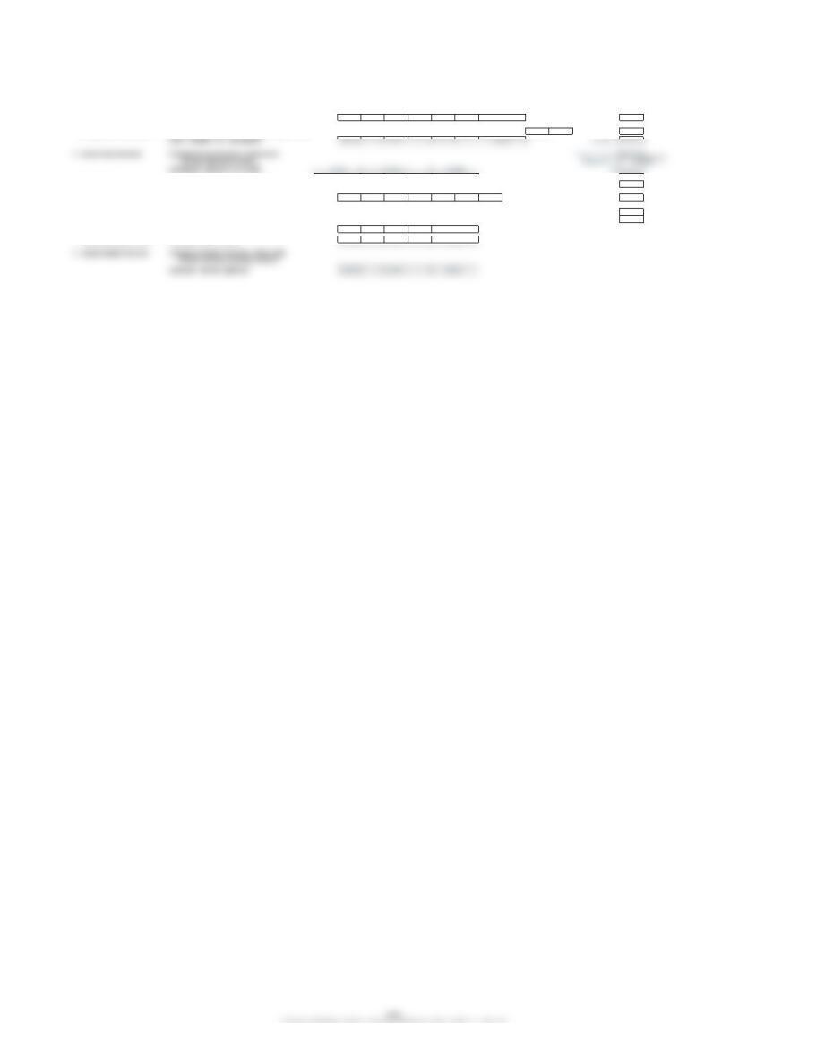
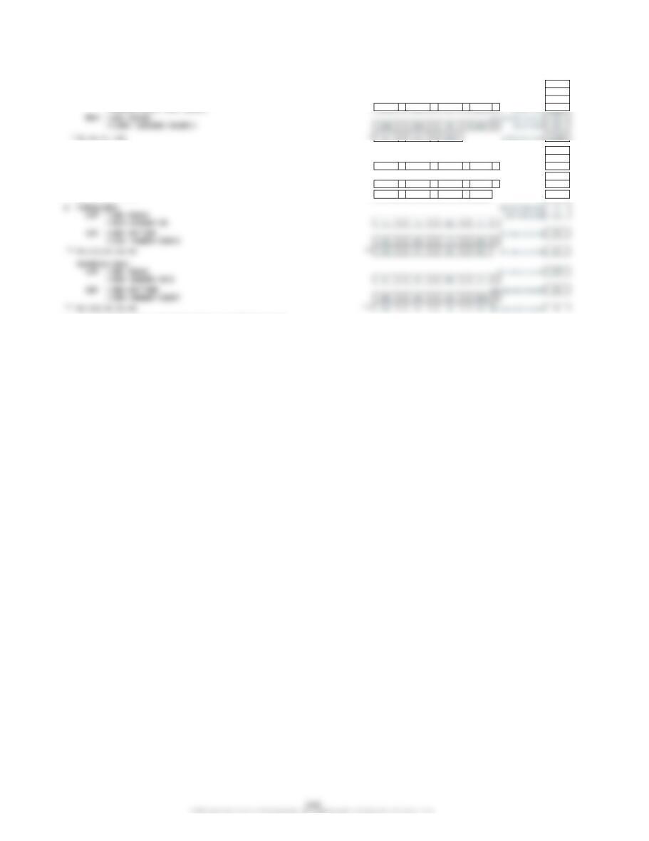
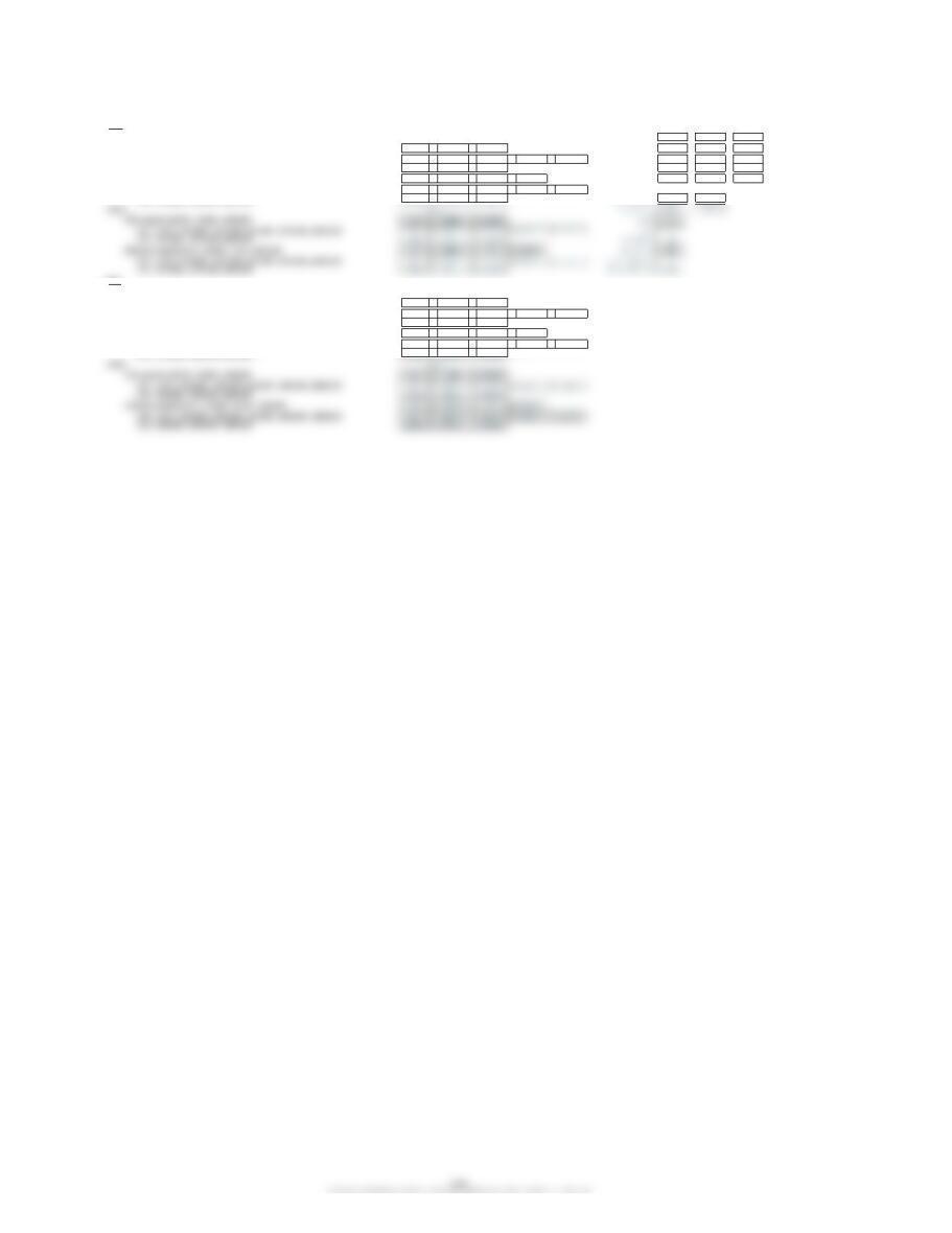
1. Fixed Overhead Rate = $832,500/450,000* = $1.85 per DLH 832,500 / 450,000 = 1.85 No. of power drills 600,000
SH = 594,000 units × 0.75 direct labor hour = 445,500 hours 594,000 × 0.75 = 445,500 Std labor hrs per drill 0.75
Applied FOH = $1.85 × 445,500 = $824,175 1.85 × 445,500 = 824,175 total budgeted OH 1,777,500
*Budgeted Hours = 600,000 units × 0.75 direct labor hours = 450,000 hours *600,000 × 0.75 = 450,000 total budgeted FOH 832,500
2. Fixed overhead analysis: Actual FOH: Actual production (units) 594,000
Budgeted FOH: 3,100 U Spending Actual DLH 446,000
1.85 × 600,000 × 0.8 Actual variable OH 928,000
835,600
Actual FOH
$835,600
$3,100 U
Spending
Budgeted FOH
$1.85 × 450,000
$832,500
$8,325 U
Applied FOH
$1.85 × 445,500
$824,175
3. Variable OH Rate = ($1,777,500 – $832,500)/450,000 hours 1,777,500 – 832,500 / 450,000 = 2.10
= $2.10 per DLH
4. Variable overhead analysis:
Actual VOH:
2. AH × SFOR: (8,600) F Spending
2.10 × 446,000 = 936,600
3. SH × SFOR: 1,050 U Efficiency
2.10 × 445,500 = 935,550
928,000
Actual VOH
112,400
Budgeted VOH:
Actual VOH
831,000
$112,400
$1,170 U
Spending
Budgeted VOH
$0.70 × 158,900
$111,230
$210 F
Efficiency
Applied VOH
$0.70 × 159,200*
$111,440
$928,000
$8,600 F
Spending
Budgeted VOH
$2.10 × 446,000
$936,600
$1,050 U
Efficiency
Applied VOH
$2.10 × 445,500
$935,550
CHAPTER 10 Standard Costing and Variance Analysis
E 10-60
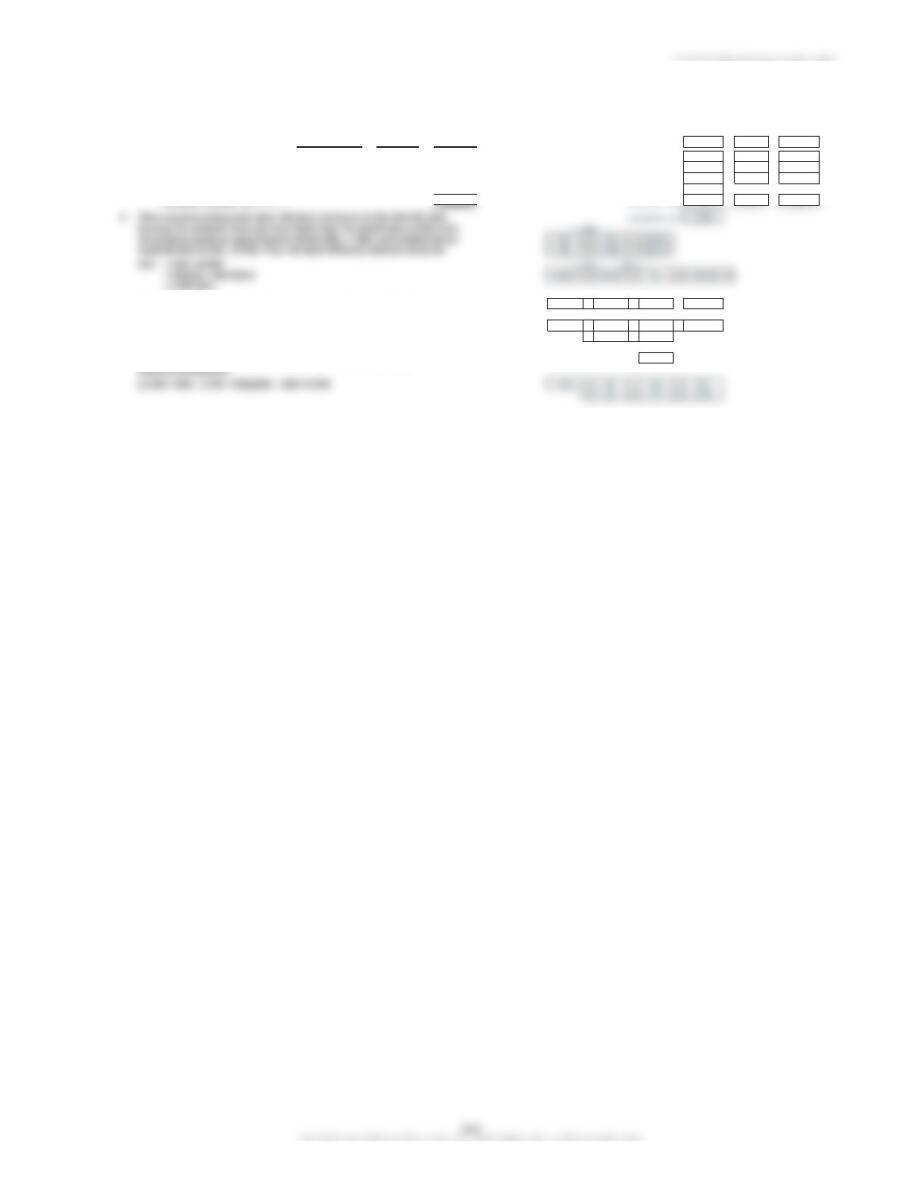
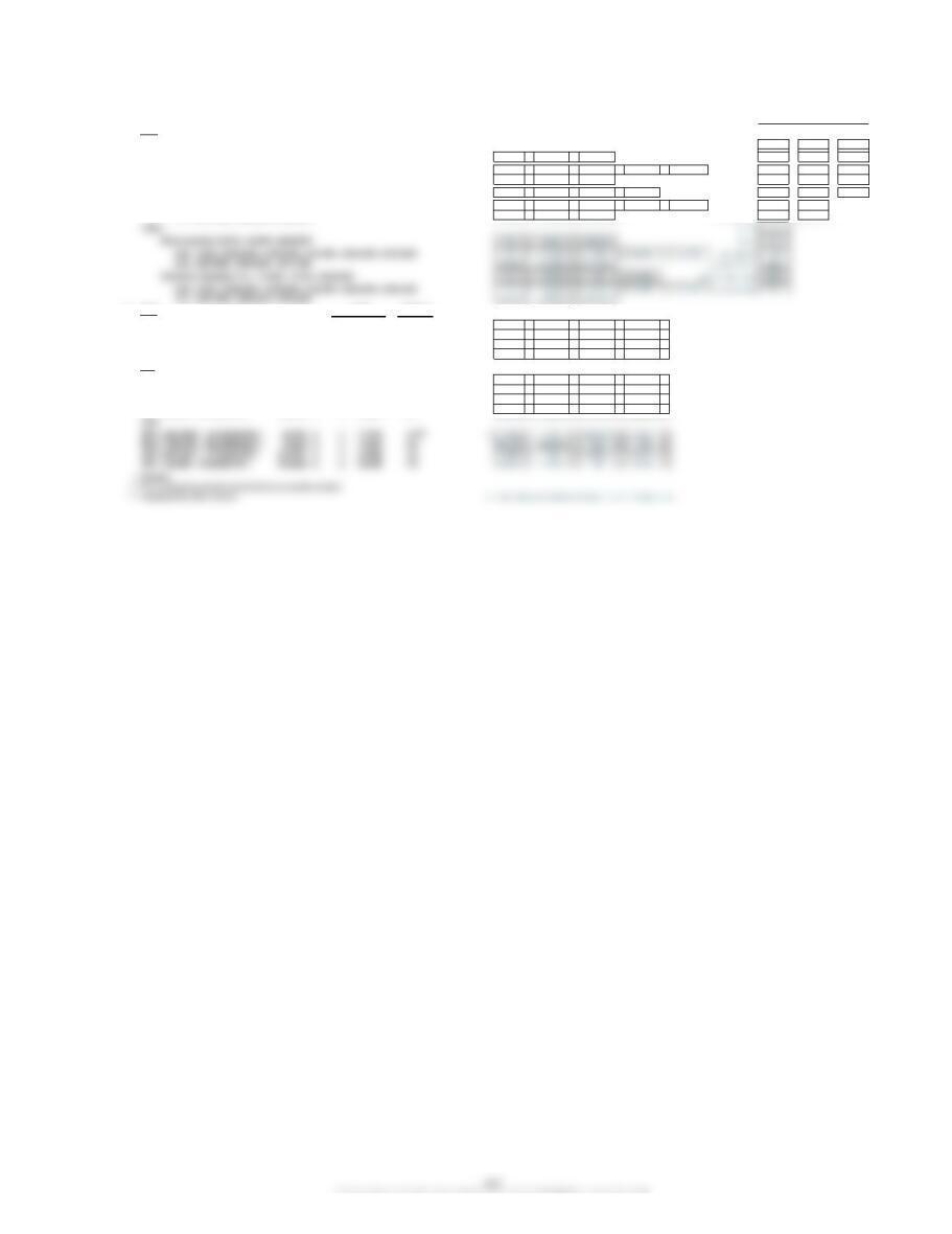
1. Total Applied Fixed Overhead
= (Standard Hours per Unit × Actual Units) × SFOR ↓ links ↓ change here, please ↓
= (0.9 × 143,000) × $11 = $1,415,700 0.9 × 143,000 × 11 = Actual units 143,000
2. Budgeted Fixed Overhead = (Standard Hours per Unit × Budgeted Units) × SFOR 29,700 U Std. units 140,000
= (0.9 × 140,000) × $11 = $1,386,000 140,000 × 0.9 × 11 = Std. labor hrs. 0.9
3. Actual Fixed Overhead = Budgeted Fixed Overhead + Unfavorable Budgeted variable OH 801,360
Overhead Spending Variance
= $1,386,000 + $24,000 = $1,410,000 + 24,000 = rate 11.00
1,386,000
1,386,000
1,386,000
1,410,000
4. Total Applied = (Standard Hours per Unit × Actual Units) × SVOR SVOR 6.36
Variable Overhead
= (0.9 × 143,000) × $6.36 = $818,532 0.9 × 143,000 × 6.36 = 818,532 Unfav. OH SP variance? 24,000
5. Budgeted Variable Overhead = Applied Variable Overhead + Unfavorable Unfav. variable OH EF variance? 1,272
Based on Actual Hours
Variable Overhead Efficiency Variance
Unfavor. variable OH SP variance? 9,196
= $818,532 + $1,272 = $819,804 818,532 + 1,272 =
= $819,804/$6.36 = 128,900 819,804 /6.36 =
6. Actual Variable Overhead = Budgeted Variable Overhead + Unfavorable
Variable Overhead Spending Variance
= $819,804 + $9,196 = $829,000 819,804 + 9,196 =
829,000
128,900
1,415,700
819,804

CHAPTER 10 Standard Costing and Variance Analysis
Chapter 10 Standard Costing and Variance Analysis
E 10-61
change here, please ↓
↓
Actual Variable
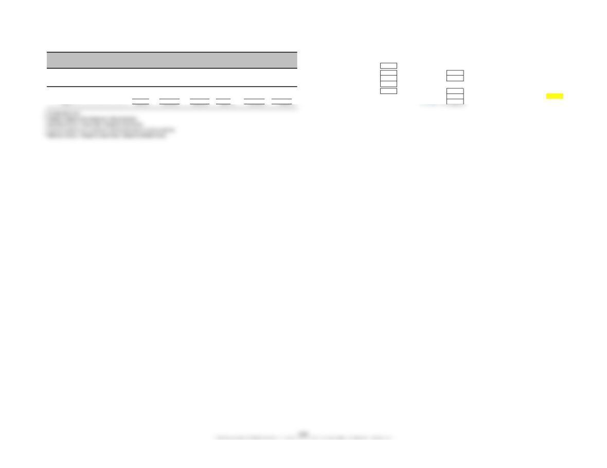
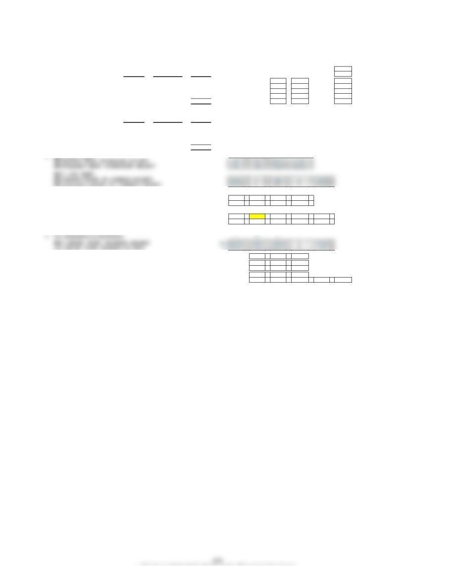
Indirect labor 36,000 Indirect labor
Supplies 3,800 hrs. reqd. 0.15
Cost Actual Actual Standard Actual hours worked 1,490 Wage rate 24.0
FormulaaCost HoursbHoursdUnits produced 10,000 Supplies
Indirect labor………………………………………………………………………………………………………………………………..
$24.00 $36,000 $35,760 $240 U$36,000 $(240) F Hours allowed 1,500 hrs. reqd. 0.15
Supplies………………………………………………………………………………………………………………………………..
2.40 3,800 3,576 224 U3,600 (24) F production Wage rate 2.40
Anker Company
Performance Report
Cost
Spending
Variancec
Budget for
Budget for
Efficiency
Variancee
For the Year Ended December 31

Chapter 10 Standard Costing and Variance Analysis
CHAPTER 10 Standard Costing and Variance Analysis
P 10-62
1. a. The managers of each cost center should be involved in setting standards.
They understand the actual conditions and are the primary source for
information on quantity used and wages paid. The newly designated
materials purchasing manager is the information source for material
prices. Since this is a new position, that individual may not have much
information to share, and Annette should go directly to those that did the
purchasing in the past. The accounting department, in conjunction with
Production, should be able to develop standards and should provide
information about past prices and usage.
waste, breakdowns, etc. Market prices for materials as well as labor
(unions) should be a consideration for setting standards.
2. Once the standards are set, actual results can be compared with the standards
and variances can be calculated. Of course, the variances themselves are only
indicators of potential problems. The underlying causes of the variances must
be determined to decide whether or not corrective action is needed. For this
reason, responsibility for the variances will be assigned to those with the most
information about them. The variances that will most likely be calculated are:
Materials Purchase Price Variance—responsibility for this variance lies with
the supervisor who was designated the materials purchasing manager. This
individual can explain why materials prices were or were not equal to the
standard amounts.
Materials Usage Variance—responsibility for this variance lies with the
manager in charge of the production department. This individual knows how
much was produced and whether or not the amount of materials used equaled
the standard.
Labor Rate Variance—responsibility for this variance lies with the manager in
charge of the production department. Again, this individual knows whether
or not the wage rate used equaled the standard.
Labor Usage Variance—responsibility for this variance lies with the manager
in charge of the production department. This individual knows how much was
produced and whether or not the amount of labor used equaled the standard.
PROBLEMS
CHAPTER 10: Standard Costing and Variance Analysis
P 10-63 ↓ links ↓
change here, please →
1. Materials: AP × AQ: Std. Qty. Std. price Std. cost
3.55
×
69,000
=
244,950 Direct materials 12 3.50 42.00
SP × AQ: 3,450 U Price Direct labor 1.7 11 18.7
3.50
×
69,000
=
241,500 Variable overhead 1.7 3 5.1
SP × SQ: 10,500 F Usage Units produced 6,000
3.50
×
72,000
=
252,000 105,000
The new process saves 0.25 × 6,000 × $3.50 = $5,250. The decision to use the 0.25
×
6,000
×
3.50
=
5,250 Actual labor costs 118,800
higher-quality material is a trade-off between the higher material cost (price
variance) and the usage variance caused by the higher-quality material. Thus,
the net savings attributable to the higher-quality material is $5,250 – $3,450 = Actual labor hours 10,800
$1,800. Keep the higher-quality material! 10,500
–
5,250
–
3,450
=
1,800 Materials purchased and used 69,000
×
=
×
=
×
=
–
=
×
=
$118,800
$0
$112,200
$6,600 U
Efficiency
Rate
$118,800
AR × AH
$11 × 10,800
SR × AH
$11 × 10,200
** SH = 1.70 × 6,000 = 10,200 ** 1.70
×
6,000
=
10,200
3. Labor for new process, 1 week later: AR × AH: 99,000
SR × AH: 0Rate
11
×
9,000
=
99,000
SR × SH: (13,200) F Efficiency
11
×
10,200
=
112,200
×
=
+
=
×
×
+
–
=
SP × SQ*
$3.50 × 72,000
$3,450 U
$10,500 F
AP × AQ
$3.55 × 69,000
SP × AQ
$3.50 × 69,000
$252,000
$244,950
$241,500
Efficiency
AR × AH
SR × AH
SR × SH
Rate
$11 × 9,000
$0
$13,200 F
$11 × 10,200
$99,000
$99,000
$112,200
Price
Usage
CHAPTER 10 Standard Costing and Variance Analysis
change here, please →
P 10-64 Granite, per square foot 50.00
1. Granite: Glue 1.50
MPV
= Actual Cost – (AQ × SP) ↓ links ↓ links ↓ Cutting labor 1.50
MUV
Glue: Act. hrs cutting labor 180
MPV
= Actual Cost – (AQ × SP) Glue purch., used 2,560
= $2,560 – (16,000 × $0.15) = $160 U 2,560 – 16,000 × 0.15 = 160 U Sq. ft. per granite 1,640
MUV
= (AQ – SQ**)SP Act. hrs install. labor 390
= (16,000 – 16,000)$0.15 = $0 16,000 – 16,000 × 0.15 = 0 Oz. glue purchased 16,000
** SQ = 50 × 32 × 10 = 16,000 ** 50 × 32 × 10 = 16,000 Std. price of glue 0.15
LRV
LEV
LRV
LEV
3. It would probably not be worthwhile for Charlene to establish standards
for every different type of installation. Tom and Tony have a small enough
operation that they can mentally decide whether or not another type of
installation (e.g., one with multiple sink cuts) will be more expensive than
the typical one.
P 10-65
change here, please →
1. Standard Standard Units Serviced Cum. Av. Time pu
Usage Cost No. of vehicles requiring service 150 40 2.5
Direct materials…………………………………………………………………………………………….
$ 4 25.000 $100.00 Std. usage 25 80 2
Direct labor………………………………………………………………………………………….
15 0.768 11.52 Std.labor rate 15 160 1.6
Variable overhead………………………………………………………………………………………….
8 0.768 6.14 Std. cost 4320 1.28
Fixed overhead………………………………………………………………………………………….
12 0.768 9.22 Std. var. O/H rate 8
3.
The cumulative average time per unit is an average . For example, the first 40 / 16.0 = 2.5 0.8
40 units take an average of 2.50 hours per unit. The second 40 take an
average of 1.5 hours per unit [(80 × 2) – (40 × 2.5)]/40 = 1.5, and, therefore, 80 × 2 – 40 × 2.5
the average for the first 80 is 2.0 per unit. Thus, as more units are produced /40 = 1.5
the cumulative average time per unit will decrease. The standard should
be 0.768 hour per unit as this is the average time taken per unit once
average time per 1st 80 units 2.0
Standard
Price
CHAPTER 10 Standard Costing and Variance Analysis
P 10-66
1. Normal delivery:
change here, please →
Standard Standard Total labor cost 580,350
Price Cost Normal Cesarean Act price per lb 9.50
Direct materials…………………………………………………………………………………………….
###### # 9.0 lbs. $ 90.00 Direct materials (lbs.) 921 Std price per lb 10.00
Direct labor………………………………………………………………………………………….
16.00 2.5 hrs. 40.00 Nursing labor (hrs.) 2.5 5 Std labor rate 16.00
Variable overhead………………………………………………………………………………………….
30.00 2.5 hrs. 75.00 Patient days 4,000 8,000 Var. O/H rate 30
Fixed overhead………………………………………………………………………………………….
40.00 2.5 hrs. 100.00 DM purchased 35,000 165,000 Fixed O/H rate 40
Unit cost………………………………………………………………………………………….
$305.00 Nursing labor (hrs.) 10,200 40,500 11.45
Cesarean delivery:
Standard Standard
Price Cost
Direct materials…………………………………………………………………………………………….
###### # 21.0 lbs. $210.00
Direct labor………………………………………………………………………………………….
16.00 5 hrs. 80.00
Variable overhead………………………………………………………………………………………….
30.00 5 hrs. 150.00
Fixed overhead………………………………………………………………………………………….
40.00 5 hrs. 200.00
Unit cost………………………………………………………………………………………….
$640.00
–
×
=
–
×
=
–
×
×
=
–
×
×
=
3. LRV = (AR – SR)AH ↓ links ↓ links ↓
LRV (Normal) = ($11.45* – $16.00)10,200 = $46,410 F
11.45
–
16.00
×
10,200
=
(46,410) F
LRV (Cesarean) = ($11.45* – $16.00)40,500 = $184,275 F 11.45
–
16.00
×
40,500
=
(184,275) F
LEV = (AH – SH)SR
LEV (Normal) = [10,200 – (2.5 × 4,000)]$16 = $3,200 U 10,200
–
2.5
×
4,000
×
16
=
3,200 U
LEV (Cesarean) = [40,500 – (5 × 8,000)]$16 = $8,000 U 40,500
–
5
×
8,000
×
16
=
8,000 U
* ($580,350/$50,700) which is rounded to the nearest cent.
–
–
×
=
–
–
×
=
5. Answers will vary. MUV: a 35,000
+
165,000
=
200,000
b4,000
×
9
=
36,000
c21
×
8,000
=
168,000
LEV: a 40,500
+
10,200
=
50,700
b4,000
×
3
+
8,000
×
5
=
50,000
Usage
Standard
Usage
Standard
P 10-67 ↓ links ↓ links ↓
change here, please →
1. Liquid Standard = 4.5 × 250,000 × $0.40 = $450,000 4.5 × 250,000 × 0.40 = 450,000 #
Upper control limit (UCL): $495,000 or $470,000; lesser = $470,000 495,000
or
470,000 lesser = 470,000
#Direct materials:
Lower control limit (LCL): $405,000 or $430,000; lesser = $430,000 405,000
or
430,000 greater = 430,000
4Liquids 1.80
Bottle Standard = 250,000 × $0.05 = $12,500 250,000 × 0.05 = 12,500 1.8 1Bottles 0.05
UCL: $13,750 UCL: 13,750 #REF! # Direct labor 3
LCL: $11,250 LCL: 11,250 1125000 Std wage rate per hr. 15.00
Direct Labor Standard = 0.2 × 250,000 × $15.00 = $750,000 0.20 × 250,000 × 15.00 = 750,000 #
ne bottles purchased
4
UCL: $825,000 or $770,000; lesser = $770,000 825,000
or
770,000 lesser = 770,000
0
nvestigation lesser of
20,000
LCL: $675,000 or $730,000; lesser = $730,000 675,000
or
2. Total Liquid Variance = $567,000 – $450,000 = $117,000 U 567,000 – 450,000 = 117,000 U Ounces of liquid purchased 1.35
The liquid variances would be investigated as the total variance exceeds 9168 0Price per bottle 0.048
The bottle variances would not be investigated as the total variance is Std price per oz. 0.40
within the accepted limits. ↓ links ↓ links ↓ Std. hrs required per bottle 0.20
3. Total Labor Variance = $733,000 – $750,000 = $17,000 F 733,000 – 750,000 = (17,000) F ?1,125,000
LRV = ($15.19* – $15.00)48,250 = $9,168 U
15.19 – 15.00 × 48,250 = 9,168 U 10%
LEV = (48,250 – 50,000)$15.00 = $26,250 F
48,250 – 50,000 × 15.00 = (26,250) F
The total variance is within the limits. However, the labor efficiency
variance is greater than $20,000 and should be investigated.
CHAPTER 10 Standard Costing and Variance Analysis
P 10-68
change here, please →
1.
April (UCL = Upper control limit, and LCL = Lower control limit) April May June
Materials: ↓ links ↓ Production (units) 90,000 100,000 110,000
Price standard: $0.25 × 723,000 = $180,750 0.25
×
723,000
=
180,750 DM Cost 189,000 218,000 230,000
UCL: (0.08 × $180,750) + $180,750 = $14,460 + $180,750 = $195,210 8%
×
180,750
=
14,460
+
180,750
=
195,210 DM Usage (lbs.) 723,000 870,000 885,000
LCL: ($14,460) + $180,750 = $166,290
14,460
+
180,750
=
166,290 DL Cost 270,000 323,000 360,000
Quantity standard: 8 × 90,000 × $0.25 = $180,000 8
×
90,000
×
0.25
=
180,000 DL Usage (hrs.) 36,000 44,000 46,000
UCL: (0.08 × $180,000) + $180,000 = $14,400 + $180,000 = $194,400 8%
×
180,000
=
14,400
+
180,000
=
194,400
LCL: ($14,400) + $180,000 = $165,600
+
=
×
=
×
=
+
=
LCL: ($21,600) + $270,000 = $248,400
+
=
×
×
=
×
=
+
=
LCL: ($21,600) + $270,000 = $248,400
+
May
Materials: ↓ links ↓
Price standard: $0.25 × 870,000 = $217,500 0.25
×
870,000
=
217,500
UCL: (0.08 × $217,500) + $217,500 = $17,400 + $217,500 = $234,900 8%
×
217,500
=
17,400
+
217,500
=
234,900
LCL: ($17,400) + $217,500 = $200,100
17,400
+
217,500
=
200,100
Quantity standard: 8 × 100,000 × $0.25 = $200,000 8
×
100,000
×
0.25
=
200,000
UCL: (0.08 × $200,000) + $200,000 = $16,000 + $200,000 = $216,000 8%
×
200,000
=
16,000
+
200,000
=
216,000
LCL: ($16,000) + $200,000 = $184,000
+
=
×
=
×
=
+
=
LCL: ($26,400) + $330,000 = $303,600
+
=
×
×
=
×
=
+
=
LCL: ($24,000) + $300,000 = $276,000
+
=
CHAPTER 10: Standard Costing and Variance Analysis
P 10-68 (Continued)
June April May June
Materials: ↓ links ↓ Production (units) 90,000 100,000 110,000
Price standard: $0.25 × 885,000 = $221,250 0.25 × 885,000 = 221,250 DM Cost 189,000 218,000 230,000
UCL: (0.08 × $221,250) + $221,250 = $17,700 + $221,250 = $238,950
8% × 221,250 = 17,700 + 221,250 = 238,950 DM Usage (lbs.) 723,000 870,000 885,000
LCL: ($17,700) + $221,250 = $203,550 17,700 + 221,250 = 203,550 DL Cost 270,000 323,000 360,000
Quantity standard: 8 × 110,000 × $0.25 = $220,000 8 × 110,000 × 0.25 = 220,000 DL Usage (hrs.) 36,000 44,000 46,000
UCL: (0.08 × $220,000) + $220,000 = $17,600 + $220,000 = $237,600
8% × 220,000 = 17,600 + 220,000 = 237,600
Cost of investigation
2,000 3,000
UCL: (0.08 × $345,000) + $345,000 = $27,600 + $345,000 = $372,600
UCL: (0.08 × $330,000) + $330,000 = $26,400 + $330,000 = $356,400
2. April
MPV = ($0.2614* – $0.25)723,000 = $8,242 U ± $14,460 4.6 →0.2614 – 0.25 × 723,000 = 8,242 U
MUV = (723,000 – 720,000)$0.25 = $750 U ± 14,400 0.4 723,000 – 720,000 × 0.25 = 750 U
LRV = ($7.5000 – $7.50)36,000 = $0 ± 21,600 0.0 7.50 – 7.50 × 36,000 = 0
LEV = (36,000 – 36,000)$7.50 = $0 ± 21,600 0.0 36,000 – 36,000 × 7.50 = 0
May
aClick a second time in the formula bar to show active cells.
MPV = ($0.2506* – $0.25)870,000 = $522 U ± 17,400 0.2 →0.2506 – 0.25 × 870,000 = 522 U
MUV = (870,000 – 800,000)$0.25 = $17,500 U ± 16,000 8.8 870,000 – 800,000 × 0.25 = 17,500 F
LRV = ($7.3409* – $7.50)44,000 = $7,000 F ± 26,400 (2.1) →7.3409 – 7.50 × 44,000 = (7,000) F
LEV = (44,000 – 40,000)$7.50 = $30,000 U ± 24,000 10.0 44,000 – 40,000 × 7.50 = 30,000 F
Actual**
Limit
(links to previous page)
Click in a cell to view links or calculations.a
***
***
%
%
CHAPTER 10 Standard Costing and Variance Analysis
P 10-68 (Continued)
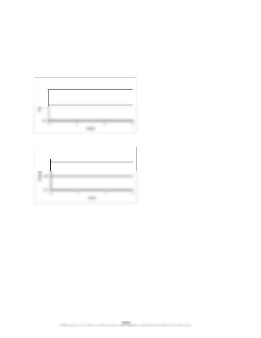
3. Control charts allow us to see when the variances are outside an
acceptable range. They may also show a pattern that might help in
pinpointing when the problem began.
Control charts: To simplify the presentation, the variances are expressed
as a percentage of the total quantity or price standard, and the y-axis is
used for variances. April (Month 1), May (Month 2), and June (Month 3)
are presented on the x-axis. These percentages were calculated in
Requirement 2.
8.0
MPV:
8.00
MUV: