217
HYPOTHESIS TESTING:
CATEGORICAL
DATA
10.1 We use the sample size formula in Equation 10.13 (in Chapter 10, text) as follows
10.2 We use Equation 10.17 (in Chapter 10, text), where drop-out rate drop-in rate .
10.3 We have
O
1 .,10 2
O
.05
218 CHAPTER 10/HYPOTHESIS TESTING: CATEGORICAL DAT
A
10.4 We use the power formula in Equation 10.14 (in Chapter 10, text) as follows:
pq 1
n
1
n
§
©
¨
¨
·
¹
¸
¸
ª
«
«
º
»
»
10.5 We have the formula
where
Thus,
CHAPTER 10/HYPOTHESIS TESTING: CATEGORICAL DATA 219
10.6 We form the 2 u 2 contingency table relating the two characteristics as follows:
received bacterial culture
received antibiotic yes no
10.7 We enumerate all possible tables with the same row and column margins.
0 7 1 6 2 5 3 4 4 3
6 12 5 13 4 14 3 15 2 16
10.9 We base the test on the discordant pairs of which there are 5 type A discordant pairs and 16 type B
discordant pairs. We wish to test the hypothesis Pr(discordant
Hp Hp p
01
1
2
1
2
::, z versus where
220 CHAPTER 10/HYPOTHESIS TESTING: CATEGORICAL DAT
A
10.12 Since there are less than 20 discordant pairs, the exact binomial version of McNemar’s test must be used.
Refer to the exact binomial tables (Table 1 in the Appendix) with to evaluate
10.13 We have the following 2 u 2 table
prior urethritis
yes no
diagnosis Gonorrhea 160 40 200
10.14 The observed table is given as follows
Association between Oracon and endometrial cancer
use Oracon
yes no
np 13 50,.
CHAPTER 10/HYPOTHESIS TESTING: CATEGORICAL DATA 221
Thus, the one-tailed p-value is given by
10.15 We display the data in the form of a 2 u 3 contingency table as follows:
genetic type
Sex
linked recessive dominant
ethnicity Engl. 46 25 54 125
222 CHAPTER 10/HYPOTHESIS TESTING: CATEGORICAL DAT
A
genetic type
Sex
linked recessive dominant
10.16 We wish to compare the diagnoses of the two doctors based on diagnoses made on the same 100 patients.
We have the following 2 u 2 table:
doctor B
+
where
Thus,
From Equation 10.23 (in Chapter 10, text),
se
N
1
n1p
e
p
e
p
2
e
a
i
b
i
a
i
b
i
ª
¼
¼
i 1
c
¦
ª
¬
Ǽ
¼
»
CHAPTER 10/HYPOTHESIS TESTING: CATEGORICAL DATA 223
10.17 We will refer to detecting fluid around the heart as a positive result, and no fluid around the heart
10.18 Let X = number of patients where the supine image is positive and the upright image is negative.
10.19 We have a point estimate = 41/75 = 0.547.
10.20 For the ear drop group, we have a point estimate for prevalence = 4/76 = 0.053.
Therefore,
10.21 We wish to test the hypothesis:
224 CHAPTER 10/HYPOTHESIS TESTING: CATEGORICAL DAT
A
10.22We form the 2 x 2 table relating outcome to group as follows:
The expected counts under the null hypothesis are as follows:
Thus, the expected table is as follows:
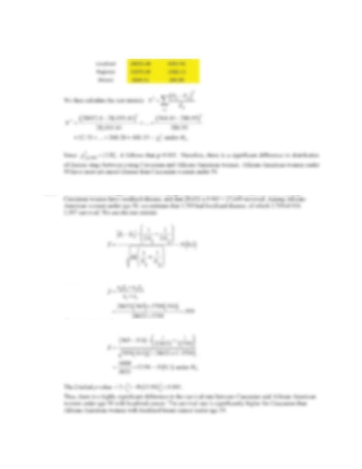
10.23 We will use a Chi-Sq test for heterogeneity. Because Table 10.23 does not give count data, we must
CaucasianAfricanͲAmerican
StageObs.ProportionObs.CountObs.ProportionObs.CountTotal
Localized0.5428652.40.463708.9832361.38
CHAPTER 10/HYPOTHESIS TESTING: CATEGORICAL DATA 225
ExpectedCount
Caucasian AfricanͲAmerican
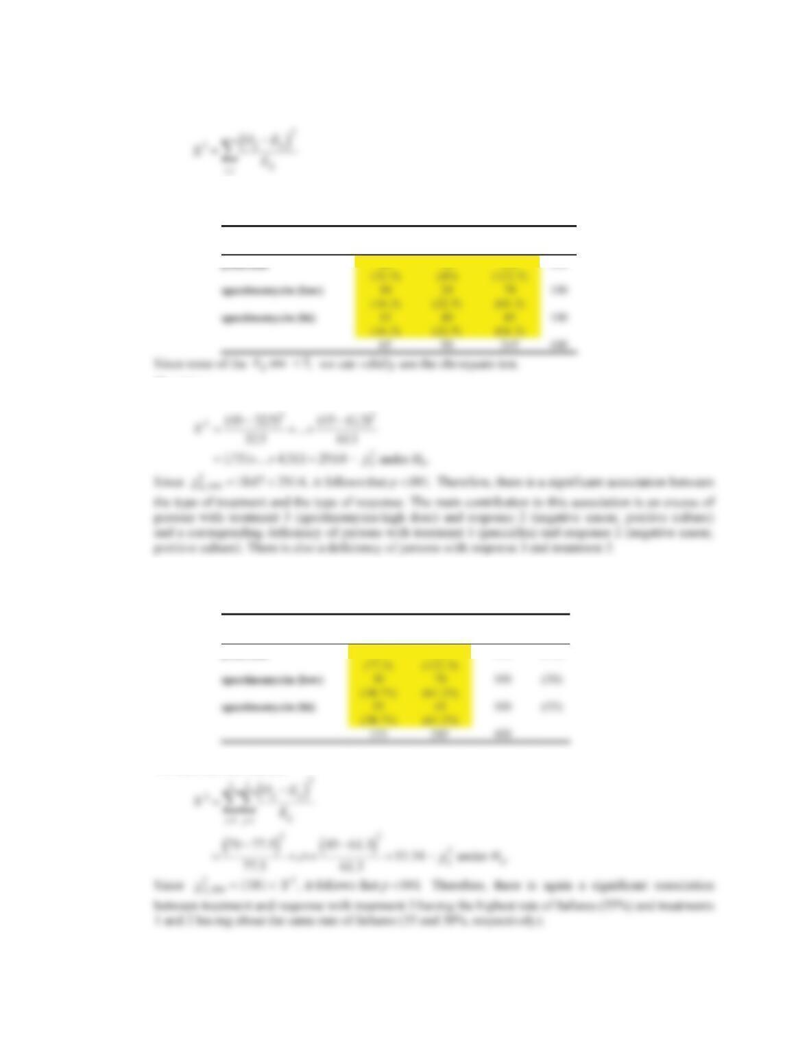
10.24 We will use a two-sample test for binomial proportions. From 10.23, we estimate that 28,652 young
where
The test statistic is then
226 CHAPTER 10/HYPOTHESIS TESTING: CATEGORICAL DAT
A
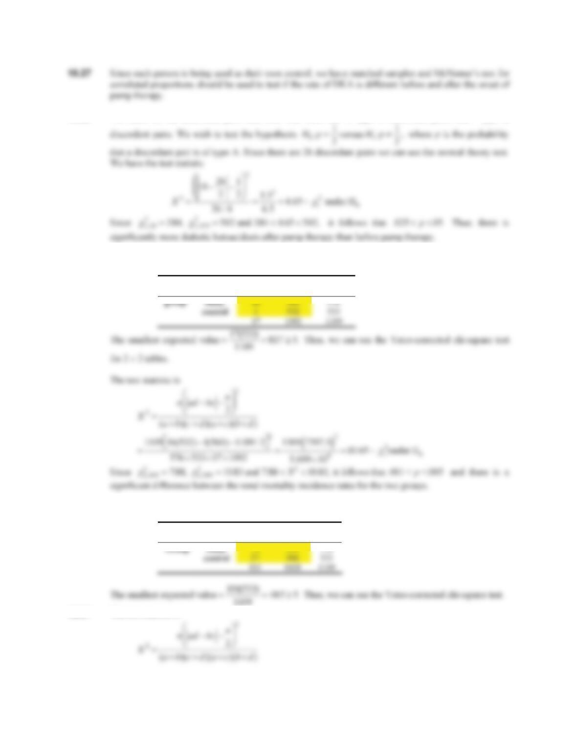
10.25 We can test for association by computing the test statistic:
We have the following in parentheses
Response
treatment + smear -sm,+cul -sm,-cul
penicillin 40
30
130
200
Therefore,
10.26 We now reduce the 3 u 3 table to a 3 u 2 table as shown below. The expected values are given in
parentheses below the observed cell counts.
Response
+
total % +
penicillin 70
130
200 (35)
We have the test statistic
OE E
ij ij ij
and with the
CHAPTER 10/HYPOTHESIS TESTING: CATEGORICAL DATA 227
10.28 We focus on the discordant pairs and note that there are 19 type A discordant pairs and 7 type B
10.29 We have the following 2 u 2 table
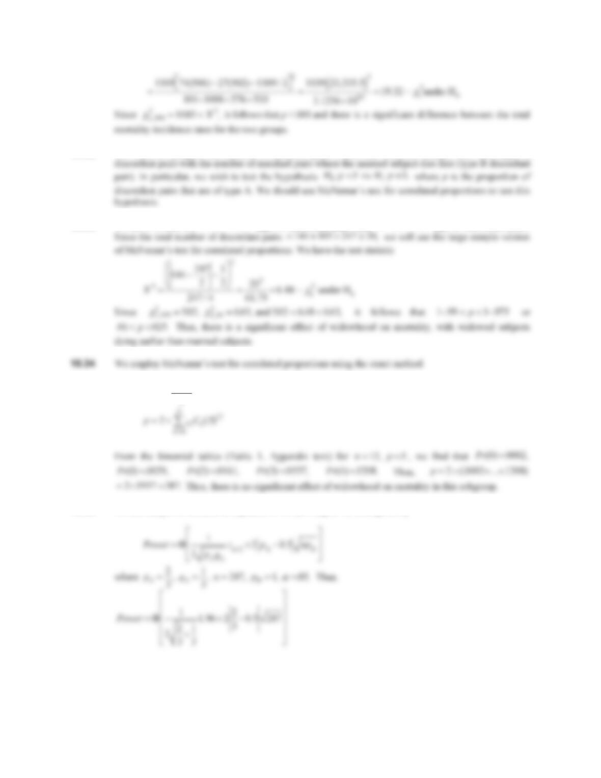
renal mortality
yes no
10.30 We have the following 2 u 2 table:
Total mortality
yes no
10.31 The test statistic is
228 CHAPTER 10/HYPOTHESIS TESTING: CATEGORICAL DAT
A
10.32 We wish to compare the number of matched pairs where the widowed subject dies first (type A
10.33 We have a total of type A discordant pairs and type B discordant pairs.
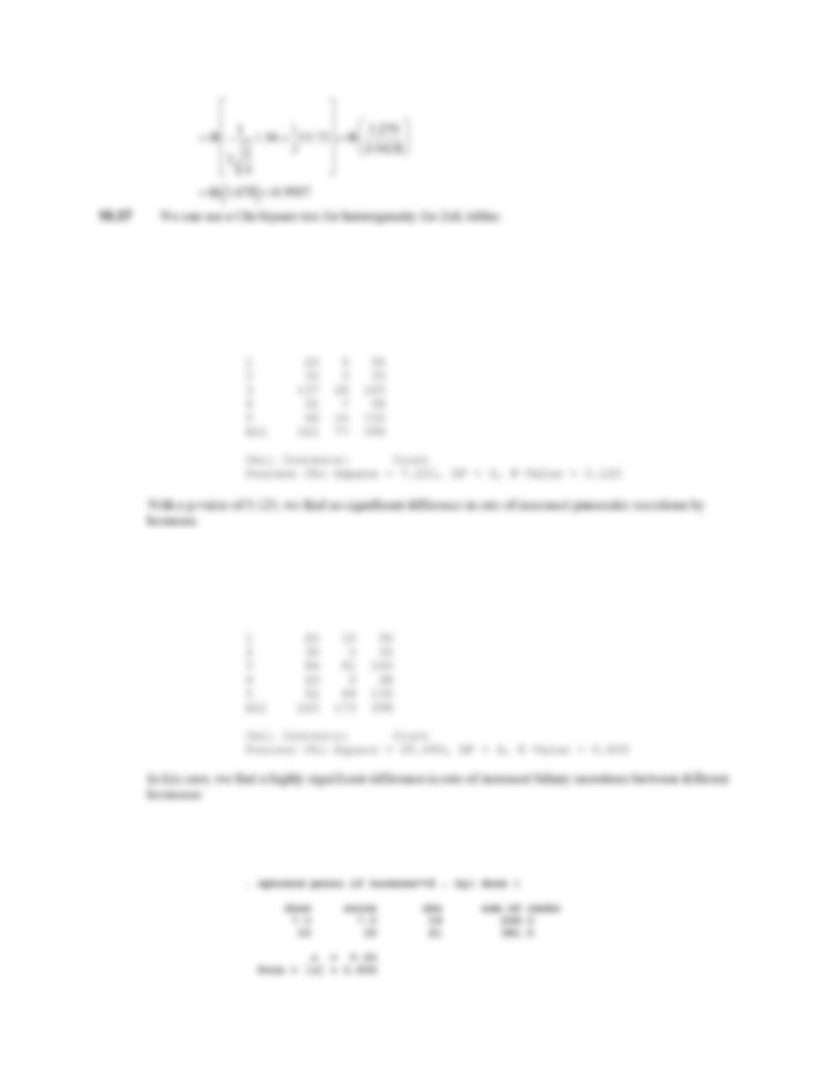
10.35 Since we compute the p-value as follows:
10.36 We use the power formula in Equation 10.16 (in Chapter 10, text) given by
87 57 144 63 40 103
aab
426,
CHAPTER 10/HYPOTHESIS TESTING: CATEGORICAL DATA 229
10.38 First we need to create an indicator variable for each observation, ‘PS inc’= if(‘Pansecpt’>’Pansecpr’,1,0),
which takes value 1 if pancreatic secretion values post > pre, and 0 otherwise. Then using MINITAB, we
can perform a Chi-Sq test with 4 df.
Tabulated statistics: Hormone, PS Inc
Rows: Hormone Columns: PS Inc
0 1 All
10.39 After creating the new variable ‘BS inc’ in a similar fashion to ‘PS inc’, we get the following results
Tabulated statistics: Hormone, BS Inc
Rows: Hormone Columns: BS Inc
0 1 All
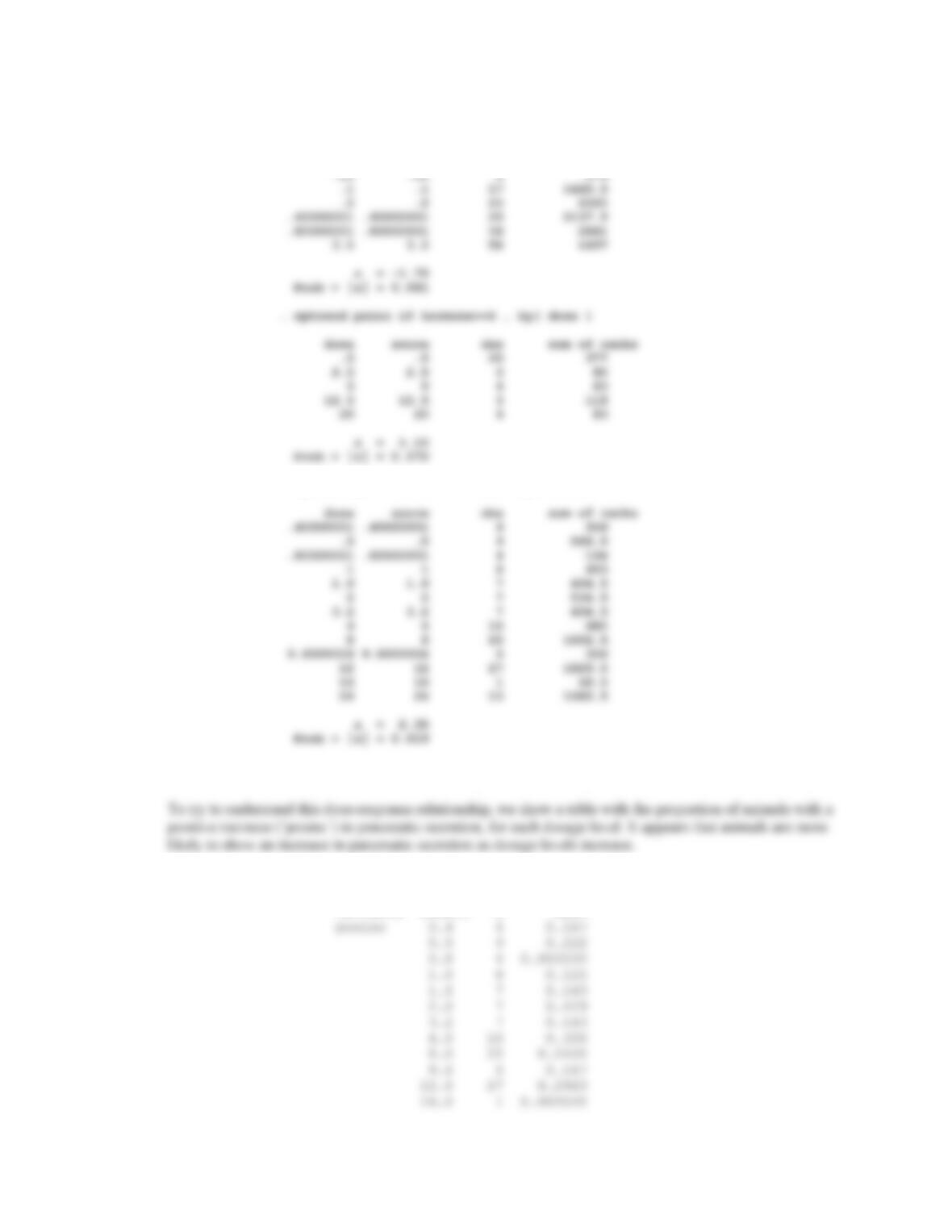
10.40 We need to use a Chi-Sq test for trend within each hormone group. In this case, it makes sense to use the
dosage level as the score value for each group. STATA will perform these trend tests with the nptrend
command. Results are shown below.
230 CHAPTER 10/HYPOTHESIS TESTING: CATEGORICAL DAT
A
. nptrend psinc if hormone==3 , by( dose )
dose score obs sum of ranks
. nptrend psinc if hormone==5 , by( dose )
Looking at pancreatic secretion, we only find a significant dose-response relation within hormone group 5.
Descriptive Statistics: posinc
Variable Dose_5 N Mean
CHAPTER 10/HYPOTHESIS TESTING: CATEGORICAL DATA 231
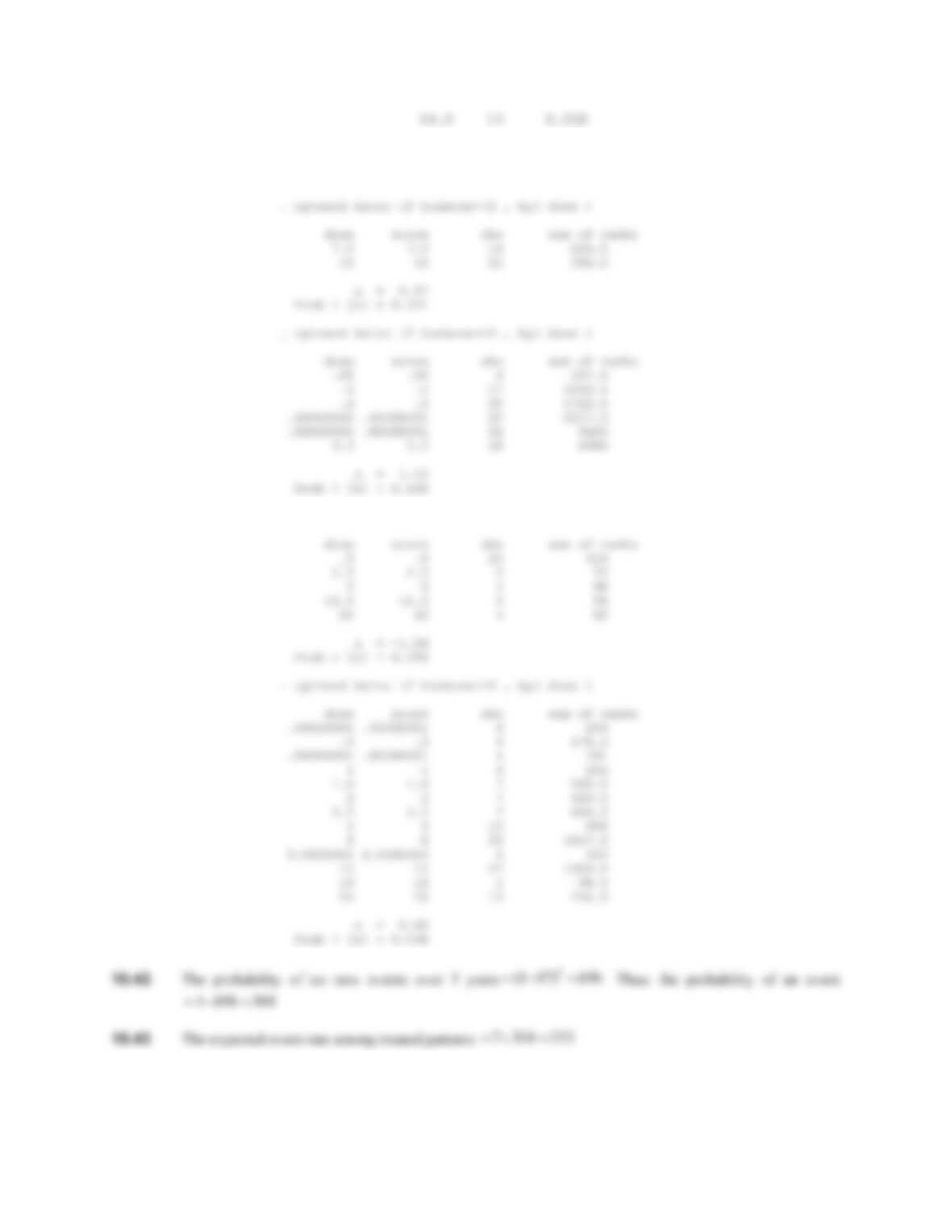
10.41 If we look at rate of increase in biliary secretion within hormone groups, we find no significant dose-
response relations for any group.
. nptrend bsinc if hormone==4 , by( dose )
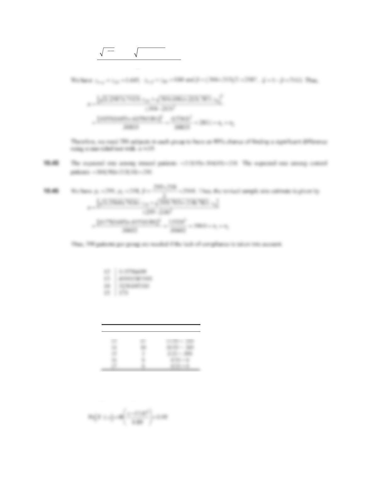
10.44 We use the sample size formula
232 CHAPTER 10/HYPOTHESIS TESTING: CATEGORICAL DAT
A
n 2pq z
1
D
/2
p
1
q
1
p
2
q
2
z
1
E
ª
¬
Ǽ
¼
»
2
‘
2
10.47 The stem-and-leaf plot is given as follows (the actual data are stem.leaf):
10.48 The total number of boys in the above plot = 33. The probability distribution of age at first developing
sperm cells is
Age Frequency Probability
12 9 9/33 = .273
10.49 We wish to find an age x such that age at spermatogenesis, which is assumed to
follow a
N13.67,0.89
2
distribution. Therefore,
Pr . .Xx Xd
95
CHAPTER 10/HYPOTHESIS TESTING: CATEGORICAL DATA 233
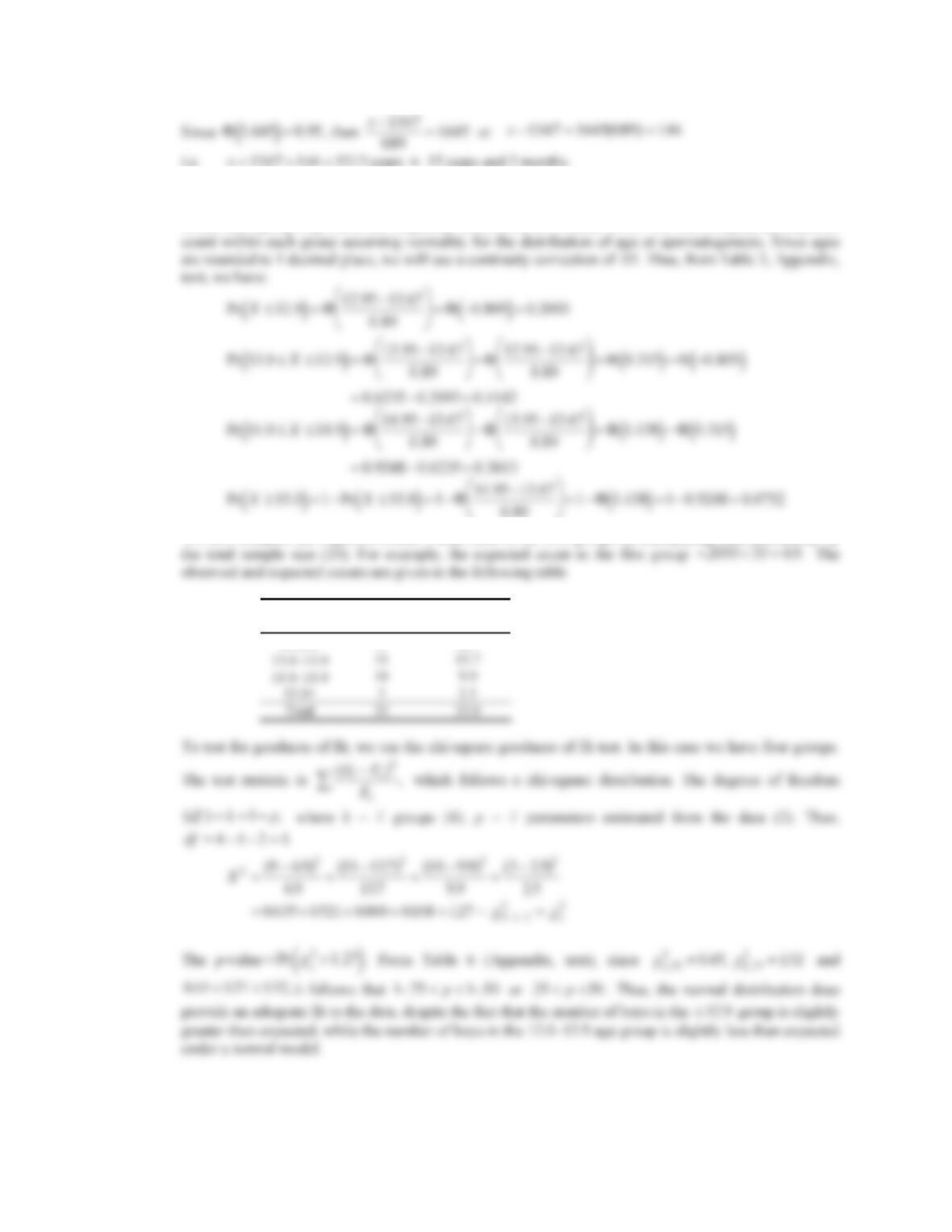
10.50 We will use the groups . The observed number of boys
within each group is given in the frequency distribution in Problem 10.63. We will compute the expected
0.89
©
¹
We now compute the expected counts within each of the four groups by multiplying each probability by
Group
Observed
Count
Expected
Count
d 12.9 9 6.9
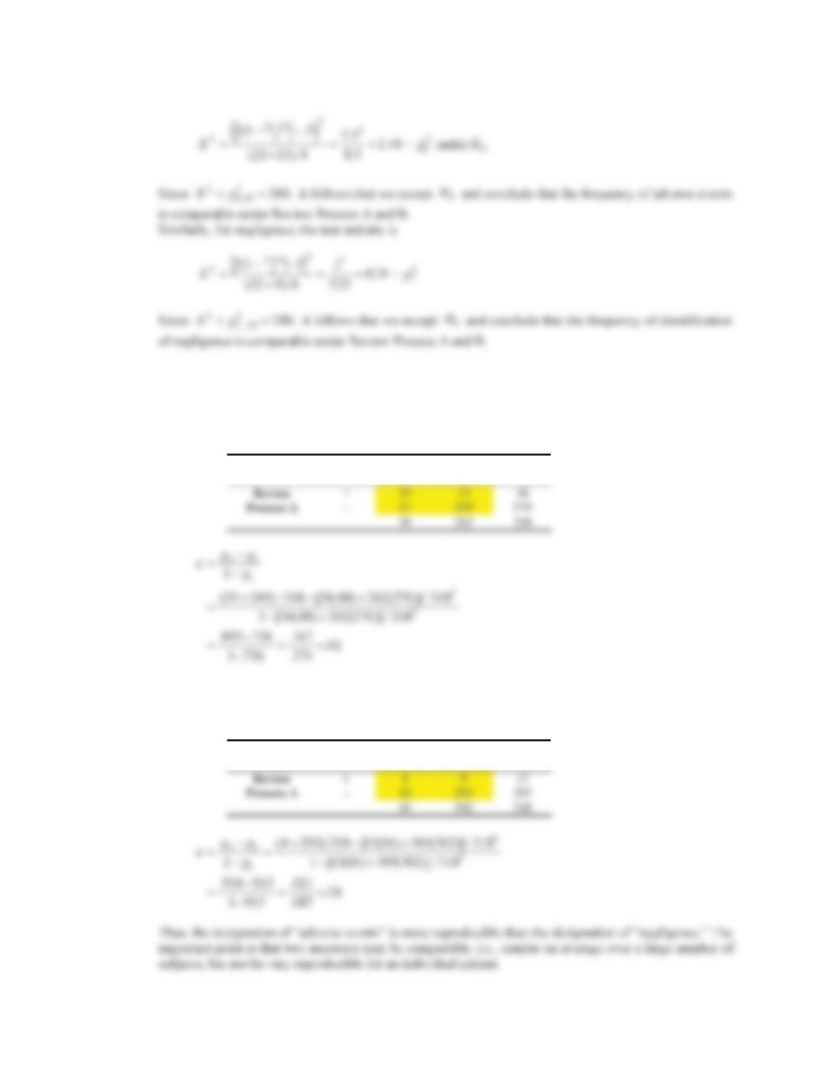
10.51 We use McNemar’s test for correlated proportions.
For adverse events, the test statistic is
12 0 12 9, 130 139, 14 0 14 9, 150 159........
234 CHAPTER 10/HYPOTHESIS TESTING: CATEGORICAL DAT
A
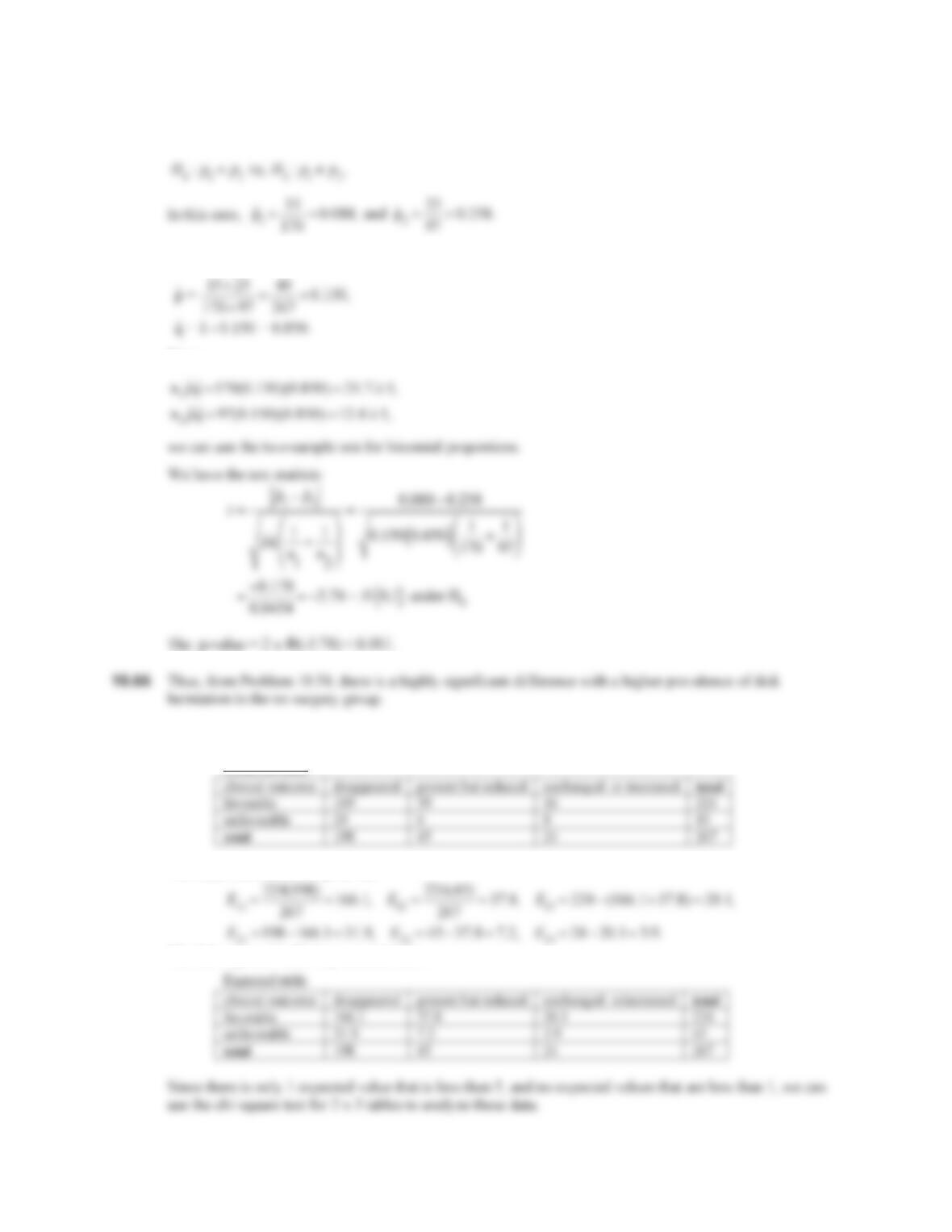
10.52 To assess reproducibility, we compute the Kappa statistic.
Adverse Events
We have the following 2 u 2 table:
Review Process B
+
Negligence
We have the following 2 u 2 table:
Review Process B
+
CHAPTER 10/HYPOTHESIS TESTING: CATEGORICAL DATA 235
10.53 We have that disk herniation was reported by 15 of the 170 patients who received surgery and 25 of the 97
patients who did not receive surgery. We wish to test the hypothesis:
10.54 We have
Since
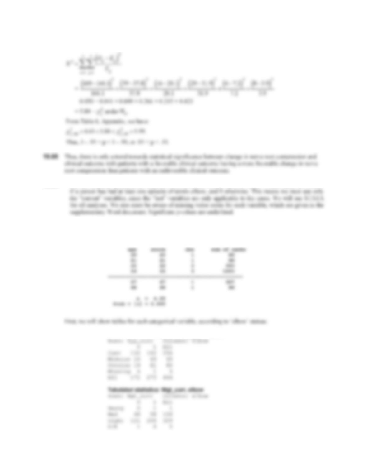
10.56 We form a 2 x 3 contingency table to represent the data as follows:
Observed table
The expected counts are given by:
The full expected table is presented below.
236 CHAPTER 10/HYPOTHESIS TESTING: CATEGORICAL DAT
A
10.57 We have the test statistic:
10.59 For this exercise, our outcome variable will be the dichotomous variable ‘elbow’, which takes the value 1
To test for an effect of age, we will use a Chi-Square test for trend.
nptrend elbow if age<99, by( age )
Tabulated statistics: Typ_curr, elbow