CHAPTER 10: Standard Costing and Variance Analysis
E 10-58
1. Variable overhead analysis:
*Standard Hours = 2 hours × 79,600 units = 159,200 hours
E 10-59
1. Fixed Overhead Rate = $832,500/450,000* = $1.85 per DLH
SH = 594,000 units × 0.75 direct labor hour = 445,500 hours
Applied FOH = $1.85 × 445,500 = $824,175
*Budgeted Hours = 600,000 units × 0.75 direct labor hours = 450,000 hours
V
4.
V
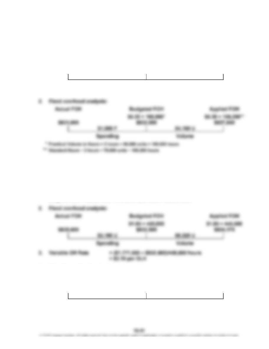
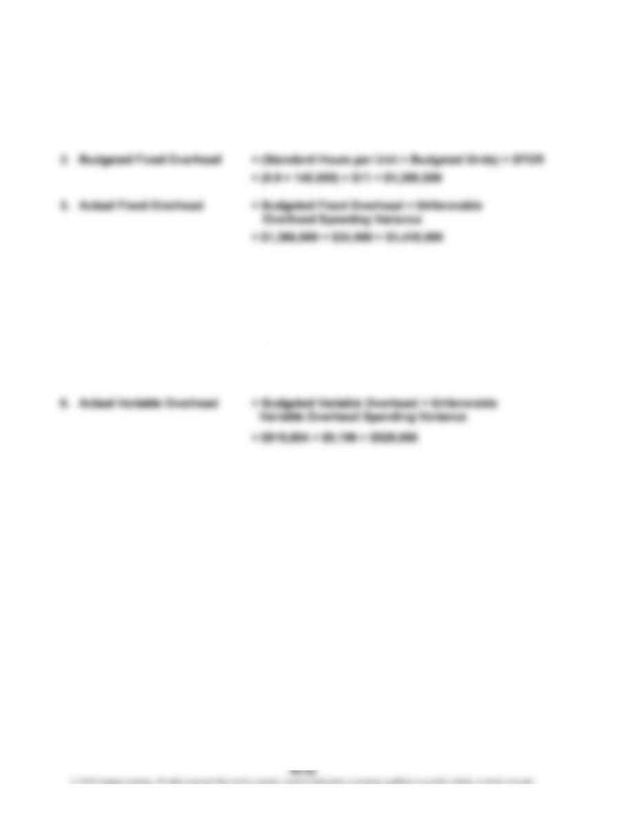
ariable overhead analysis:
$928,000
$8,600 F
Spending
Budgeted VOH
$2.10 × 446,000
$936,600
$1,050 U
Efficiency
Applied VOH
$2.10 × 445,500
$935,550
Actual VOH
$112,400
$1,170 U
Spending
Budgeted VOH
$0.70 × 158,900
$111,230
$210 F
Efficiency
Applied VOH
$0.70 × 159,200*
$111,440
Actual VOH
CHAPTER 10 Standard Costing and Variance Analysis
E 10-60
1. Total Applied Fixed Overhead = (Standard Hours per Unit × Actual Units) × SFOR
= (0.9 × 143,000) × $11 = $1,415,700
4. Total Applied = (Standard Hours per Unit × Actual Units) × SVOR
V
ariable Overhead
= (0.9 × 143,000) × $6.36 = $818,532
5. Budgeted Variable Overhead = Applied Variable Overhead + Unfavorable
Based on Actual Hours Variable Overhead Efficiency Variance
= $818,532 + $1,272 = $819,804
Actual Direct Labor Hours = $819,804/$6.36 = 128,900
V
Chapter 10 Standard Costing and Variance Analysis
E 10-61
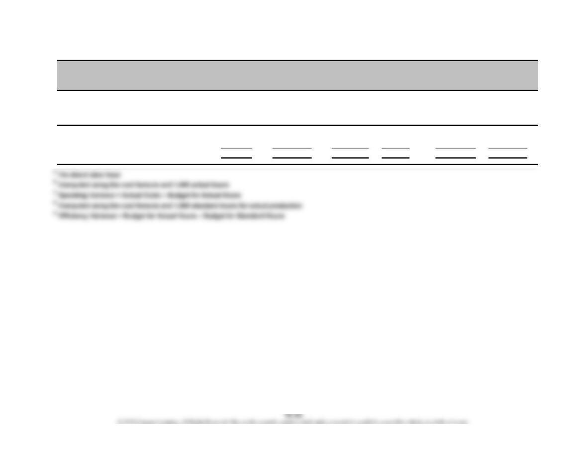
Cost Actual Actual Standard
Formula
a
Cost Hours
b
Hours
d
Indirect labor…………………………………
…
$24.00 $36,000 $35,760 $240 U $36,000 $(240) F
Supplies………………………………………
…
2.40 3,800 3,576 224 U 3,600 (24) F
Total………………………………………… $26.40 $39,800 $39,336 $464 U $39,600 $(264) F
Anker Company
Performance Report
Cost
Spending
Variance
c
Budget for Budget for
Efficiency
Variance
e
For the Year Ended December 31
CHAPTER 10 Standard Costing and Variance Analysis
P 10-62
1. a. The managers of each cost center should be involved in setting standards.
They understand the actual conditions and are the primary source fo
r
information on quantity used and wages paid. The newly designated
materials purchasing manager is the information source for material
2. Once the standards are set, actual results can be compared with the standards
and variances can be calculated. Of course, the variances themselves are only
indicators of potential problems. The underlying causes of the variances must
be determined to decide whether or not corrective action is needed. For this
reason, responsibility for the variances will be assigned to those with the most
Materials Usage Variance—responsibility for this variance lies with the
manager in charge of the production department. This individual knows how
much was produced and whether or not the amount of materials used equaled
the standard.
Labor Rate Variance—responsibility for this variance lies with the manager in
charge of the production department. Again, this individual knows whether
or not the wage rate used equaled the standard.
PROBLEMS
CHAPTER 10: Standard Costing and Variance Analysis
P 10-63
1. Materials:
2. Labor for new process:
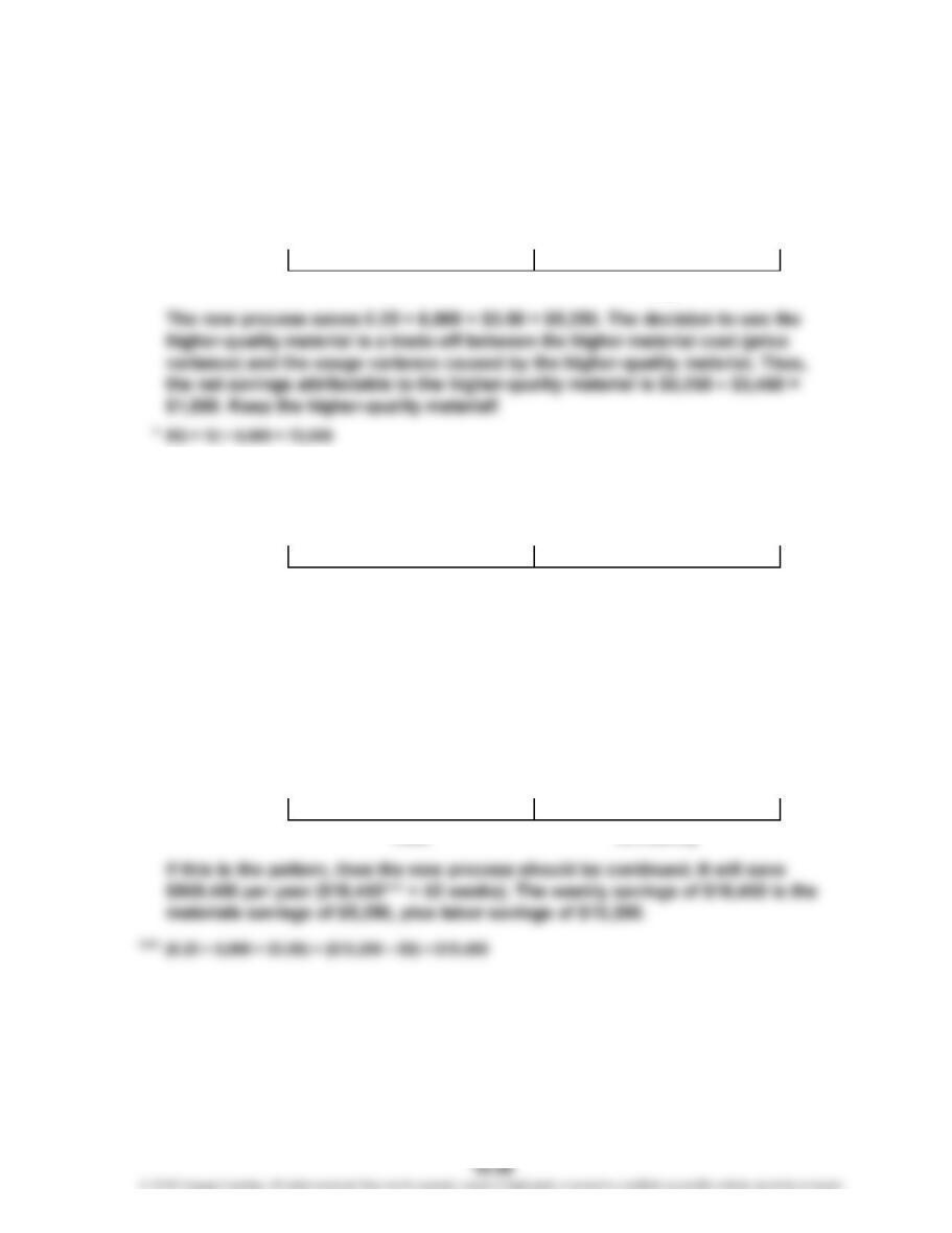
The new process saves $5,250 in materials usage (see Requirement 1) but loses
$6,600 from the labor effect, giving a net loss of $1,350. If this pattern is
expected to persist, then the new process should be abandoned.
**
SH = 1.70 × 6,000 = 10,200
3. Labor for new process, 1 week later:
$6,600 U
EfficiencyRate
$118,800
Price Usage
AR × AH
$11 × 10,800
SR × SH**SR × AH
$11 × 10,200
AR × AH SR × AH SR × SH
$118,800
$11 × 9,000
$0 $13,200 F
$11 × 10,200
$0
$112,200
$99,000 $99,000 $112,200
SP × SQ*
$3.50 × 72,000
$3,450 U $10,500 F
AP × AQ
$3.55 × 69,000
SP × AQ
$3.50 × 69,000
$252,000$244,950 $241,500
CHAPTER 10 Standard Costing and Variance Analysis
P 10-64
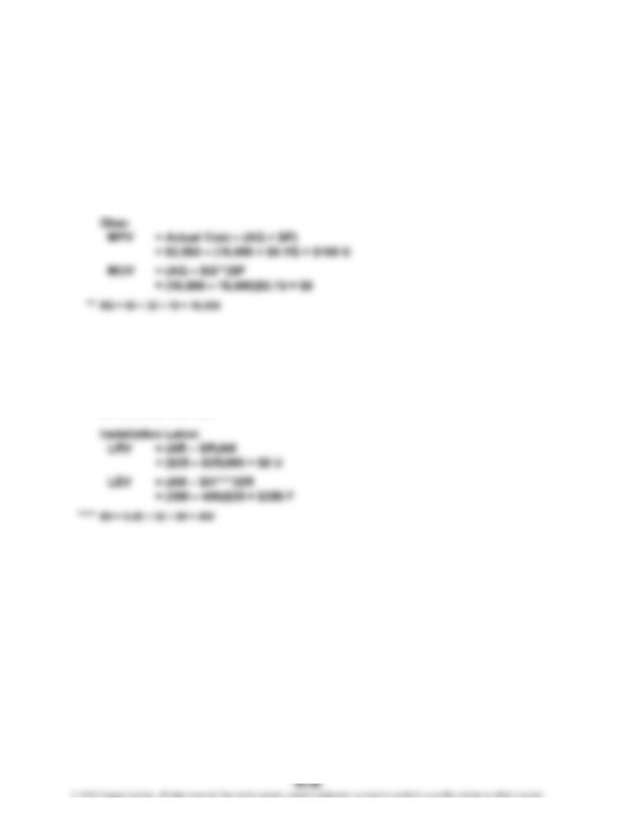
1. Granite:
MPV = Actual Cost – (AQ × SP)
= $79,048 – (1,640 × $50) = $2,952 F
MUV = (AQ – SQ*)SP
= (1,640 – 1,600)$50 = $2,000 U
*SQ = 50 × 32 = 1,600
2. Cutting Labor:
LRV = (AR – SR)AH
= ($15 – $15)180 = $0
LEV = (AH – SH***)S
R
= (180 – 160)$15 = $300 U
*** SH = 0.10 × 32 × 50 = 160
3. It would probably not be worthwhile for Charlene to establish standards
for every different type of installation. Tom and Tony have a small enough
operation that they can mentally decide whether or not another type of
installation (e.g., one with multiple sink cuts) will be more expensive than
the typical one.
CHAPTER 10: Standard Costing and Variance Analysis
P 10-65
1. Standard Standard
Usage Cost
Direct materials………………………… $ 4 25.000 $100.00
Direct labor……………………………
…
15 0.768 11.52
…
2. There would be unfavorable labor efficiency variances for the first 320 units
because the standard hours are much lower than the actual hours at this level.
Actual hours would be approximately 409.60 (320 × 1.280), and standard hours
would be 245.76 (320 × 0.768). Thus, the labor efficiency variance would be:
LEV = (AH – SH)SR
= (409.60 – 245.76)$15
= 2,457.60 U
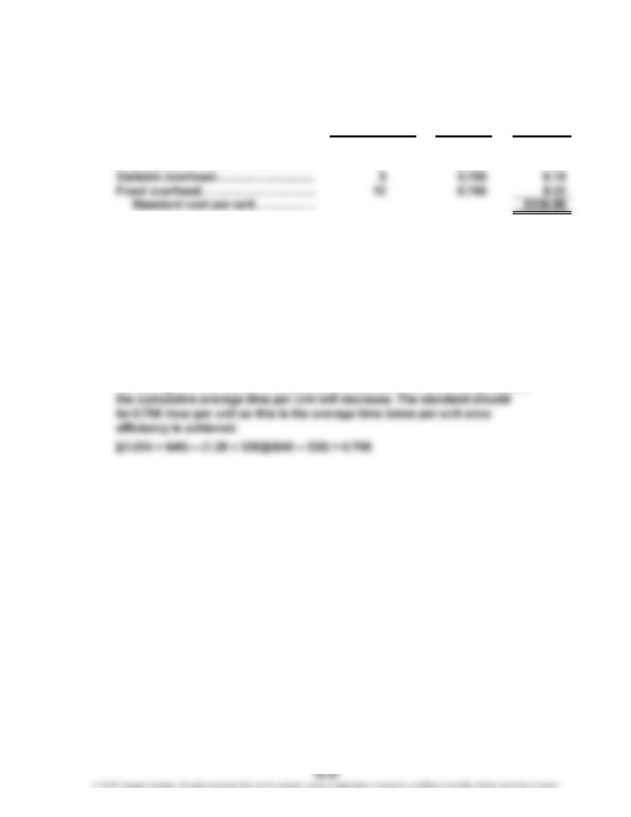
3. The cumulative average time per unit is an averag
e
. For example, the first
40 units take an average of 2.50 hours per unit. The second 40 take an
average of 1.5 hours per unit [(80 × 2) – (40 × 2.5)]/40 = 1.5, and, therefore,
the average for the first 80 is 2.0 per unit. Thus, as more units are produced
Standard
Price
CHAPTER 10 Standard Costing and Variance Analysis
P 10-66
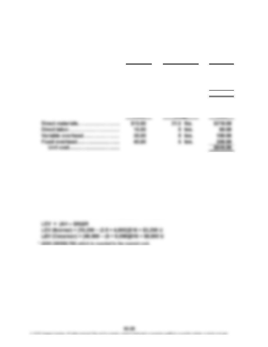
1. Normal delivery:
Standard Standard
Price Cost
Direct materials……………………
…
$10.00 9.0 lbs. $ 90.00
Direct labor…………………………
…
16.00 2.5 hrs. 40.00
V
ariable overhead…………………
…
30.00 2.5 hrs. 75.00
Fixed overhead……………………
…
40.00 2.5 hrs. 100.00
Unit cost…………………………
…
$305.00
Cesarean delivery:
Standard Standard
2. MPV = (AP – SP)AQ
MPV (Normal) = ($9.50 – $10.00)35,000 = $17,500 F
MPV (Cesarean) = ($9.50 – $10.00)165,000 = $82,500 F
MUV = (AQ – SQ)SP
MUV (Normal) = [35,000 – (9 × 4,000)]$10 = $10,000 F
MUV (Cesarean) = [165,000 – (21 × 8,000)]$10 = $30,000 F
3. LRV = (AR – SR)AH
LRV (Normal) = ($11.45* – $16.00)10,200 = $46,410 F
LRV (Cesarean) = ($11.45* – $16.00)40,500 = $184,275 F
4.
Y
es. Computations are shown below.
MUV = (200,000 – 36,000 – 168,000)$10 = $40,000 F
LEV = (50,700 – 10,000 – 40,000)$16 = $11,200 U
5. Answers will vary.
Standard
Usage
Standard
…
…
V
…
…
…
CHAPTER 10: Standard Costing and Variance Analysis
P 10-67
1. Liquid Standard = 4.5 × 250,000 × $0.40 = $450,000
Upper control limit (UCL): $495,000 or $470,000; lesser = $470,000
Lower control limit (LCL): $405,000 or $430,000; lesser = $430,000
2. Total Liquid Variance = $567,000 – $450,000 = $117,000 U
MPV = ($0.42 – $0.40)1,350,000 = $27,000 U
MUV = (1,350,000 – 1,125,000)$0.40 = $90,000 U
The liquid variances would be investigated as the total variance exceeds
$20,000, as does each individual variance.
Total Bottle Variance = $12,000 – $12,500 = $500 F
MPV = ($0.048 – $0.05)250,000 = $500 F
MUV = (250,000 – 250,000)$0.05 = $0
The bottle variances would not be investigated as the total variance is
within the accepted limits.
CHAPTER 10 Standard Costing and Variance Analysis
P 10-68
1. April (UCL = Upper control limit, and LCL = Lower control limit)
Materials:
Price standard: $0.25 × 723,000 = $180,750
UCL: (0.08 × $180,750) + $180,750 = $14,460 + $180,750 = $195,210
LCL: ($14,460) + $180,750 = $166,290
Labor:
Price standard: $7.50 × 36,000 = $270,000
UCL: (0.08 × $270,000) + $270,000 = $21,600 + $270,000 = $291,600
LCL: ($21,600) + $270,000 = $248,400
May
Materials:
Price standard: $0.25 × 870,000 = $217,500
UCL: (0.08 × $217,500) + $217,500 = $17,400 + $217,500 = $234,900
LCL: ($17,400) + $217,500 = $200,100
Quantity standard: 8 × 100,000 × $0.25 = $200,000
UCL: (0.08 × $200,000) + $200,000 = $16,000 + $200,000 = $216,000
LCL: ($16,000) + $200,000 = $184,000
P 10-68 (Continued)
June
Materials:
Price standard: $0.25 × 885,000 = $221,250
UCL: (0.08 × $221,250) + $221,250 = $17,700 + $221,250 = $238,950
LCL: ($17,700) + $221,250 = $203,550
Quantity standard: 8 × 110,000 × $0.25 = $220,000
UCL: (0.08 × $220,000) + $220,000 = $17,600 + $220,000 = $237,600
LCL: ($17,600) + $220,000 = $202,400
2. April
MPV = ($0.2614* – $0.25)723,000 = $8,242 U ± $14,460 4.6
MUV = (723,000 – 720,000)$0.25 = $750 U ± 14,400 0.4
LRV = ($7.5000 – $7.50)36,000 = $0 ± 21,600 0.0
LEV = (36,000 – 36,000)$7.50 = $0 ± 21,600 0.0
May
MPV = ($0.2506* – $0.25)870,000 = $522 U ± 17,400 0.2
MUV = (870,000 – 800,000)$0.25 = $17,500 U ± 16,000 8.8
LRV = ($7.3409* – $7.50)44,000 = $7,000 F ± 26,400 (2.1)
LEV = (44,000 – 40,000)$7.50 = $30,000 U ± 24,000 10.0
A
ctual**Limit
***
***
%
%
CHAPTER 10 Standard Costing and Variance Analysis
P 10-68 (Continued)
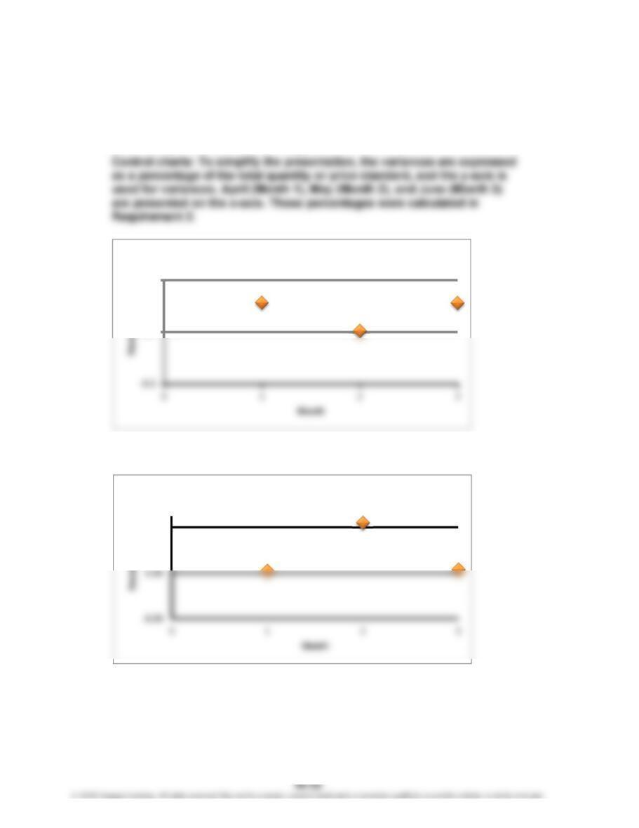
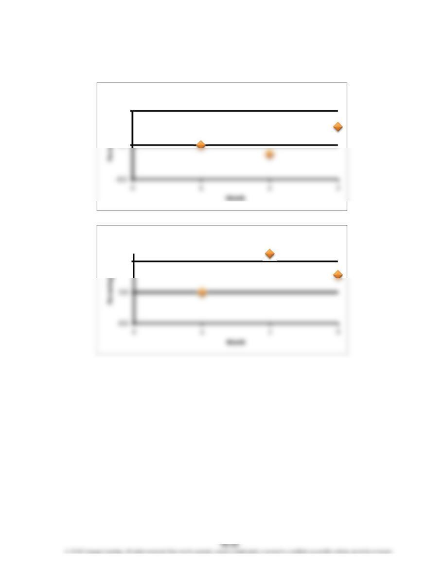
3. Control charts allow us to see when the variances are outside an
acceptable range. They may also show a pattern that might help in
pinpointing when the problem began.
8.0
MPV:
8.00
MUV:
CHAPTER 10: Standard Costing and Variance Analysis
P 10-68 (Concluded)
8.0
LRV:
8.0
LEV: