Chapter 10
Standard Costs and Variances
Solutions to Questions
10-1 A quantity standard indicates how much
of an input should be used to make a unit of
output. A price standard indicates how much the
input should cost.
10-2 Separating an overall variance into a
price variance and a quantity variance provides
more information. Moreover, price and quantity
variances are usually the responsibilities of
different managers.
10-3 The materials price variance is usually
the responsibility of the purchasing manager.
The materials quantity and labor efficiency
variances are usually the responsibility of
production managers and supervisors.
10-4 The materials price variance can be
computed when materials are purchased or
10-5 This combination of variances may
indicate that inferior quality materials were
purchased at a discounted price, but the low–
quality materials created production problems.
10-6 If standards are used to find who to
blame for problems, they can breed resentment
and undermine morale. Standards should not be
used to find someone to blame for problems.
10-7 Several factors other than the
contractual rate paid to workers can cause a
labor rate variance. For example, skilled workers
with high hourly rates of pay can be given duties
that require little skill and that call for low hourly
rates of pay, resulting in an unfavorable rate
variance. Or unskilled or untrained workers can
be assigned to tasks that should be filled by
more skilled workers with higher rates of pay,
resulting in a favorable rate variance.
Unfavorable rate variances can also arise from
overtime work at premium rates.
10-8 If poor quality materials create
production problems, a result could be excessive
labor time and therefore an unfavorable labor
efficiency variance. Poor quality materials would
not ordinarily affect the labor rate variance.
Only the “SR” part of the formula, the standard
rate, differs between the two variances.
10-10 If labor is a fixed cost in the short run
and demand is insufficient to keep everyone
busy (and workers are not laid off), it will result
in an unfavorable labor efficiency variance. To
avoid this unfavorable variance, managers may
choose to produce at capacity (rather than
reducing output to match customer demand)

which leads to a build up of work in process and
finished goods inventories.
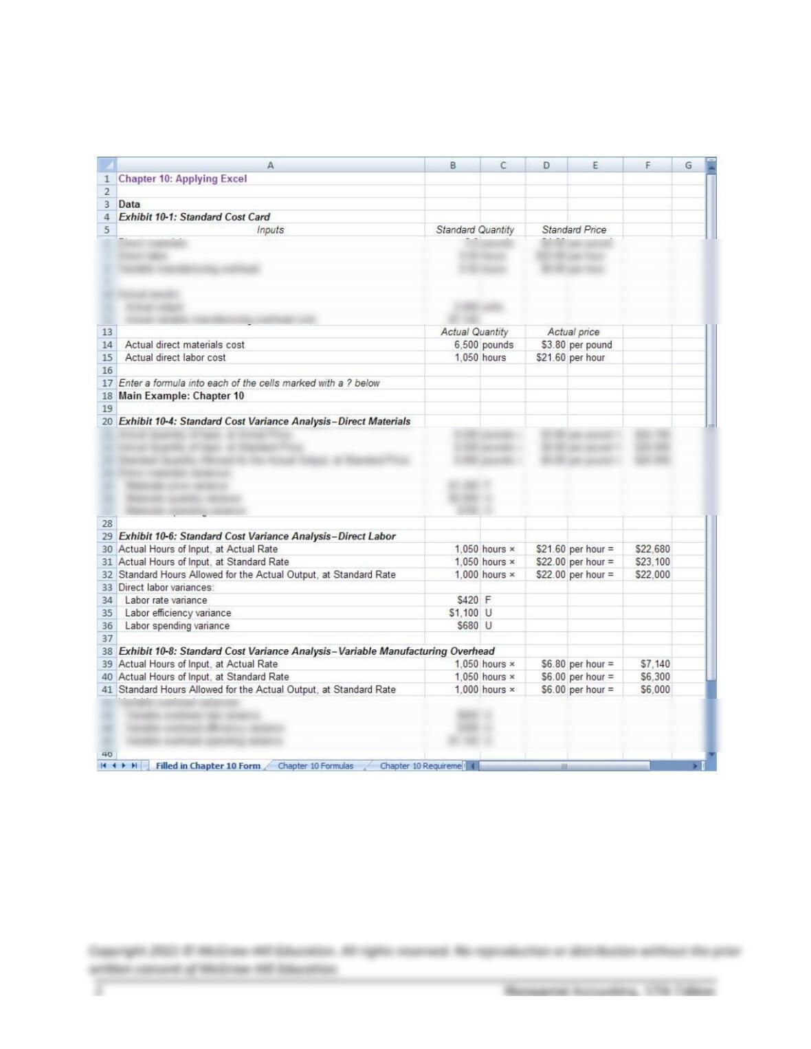
Chapter 10: Applying Excel
The completed worksheet is shown below.
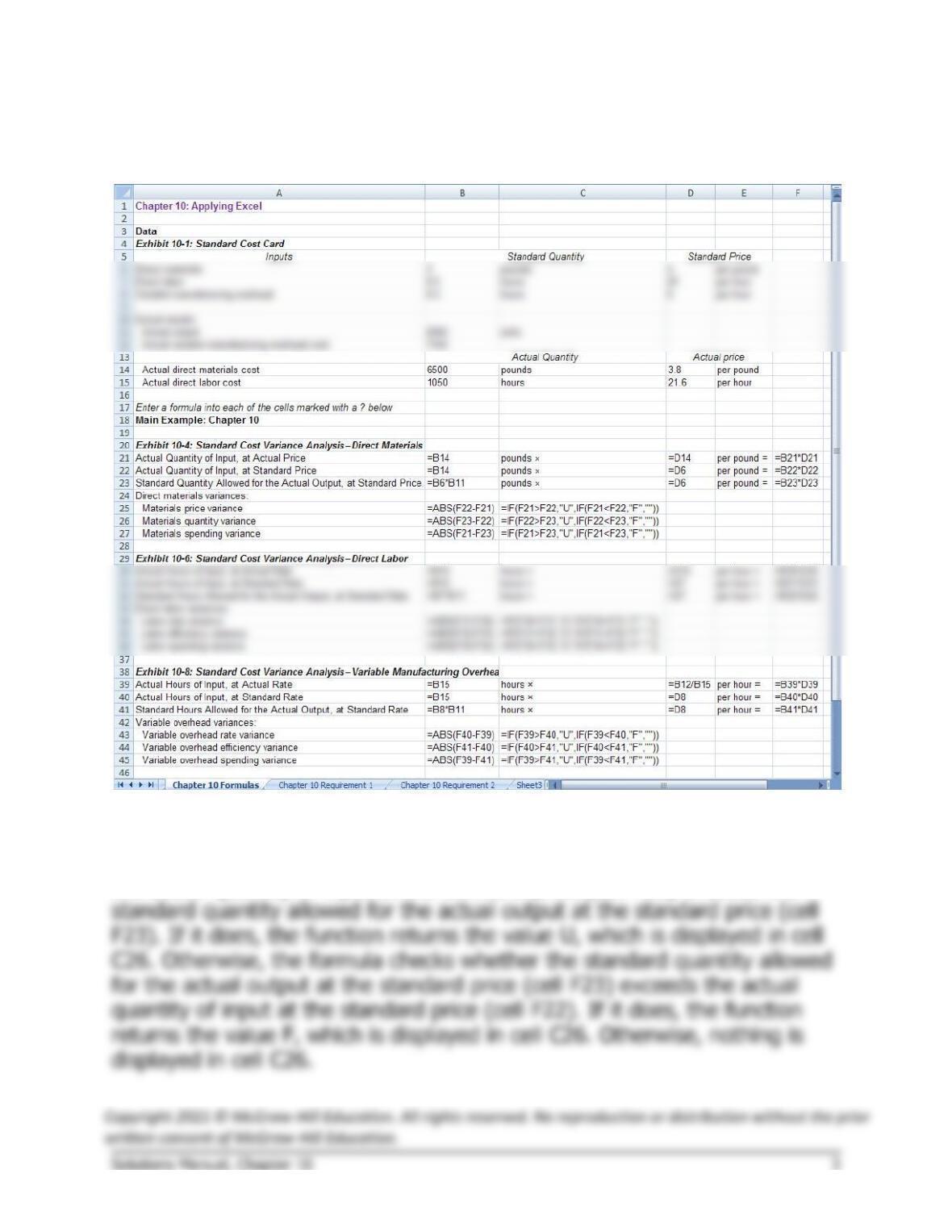
Chapter 10: Applying Excel (continued)
The completed worksheet, with formulas displayed, is shown below.
Note: The formulas to compute whether a variance is Favorable or
Unfavorable use the IF() function. For example, in cell C26, the formula is
=IF(F22>F23,”U”,IF(F22<F23,”F”,””)). This formula first checks whether
the actual quantity of input at the standard price (cell F22) exceeds the
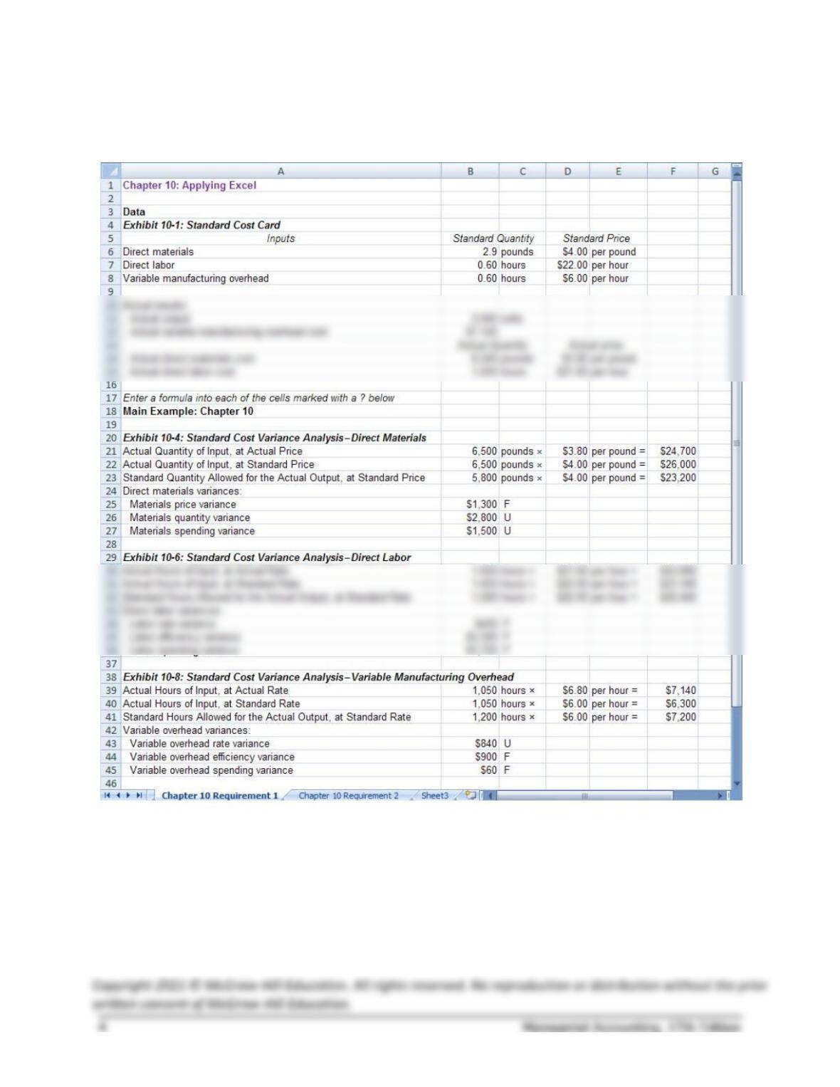
Chapter 10: Applying Excel (continued)
1. With the changes in data, the result is:
a. The materials quantity variance is $2,800 U. This variance is the
difference between the amount of materials that should have been
used to make the actual output and the actual amount of materials
used, all evaluated at the standard price. This variance is unfavorable
because 6,500 pounds were used, but 5,800 pounds should have
been used.
Chapter 10: Applying Excel (continued)
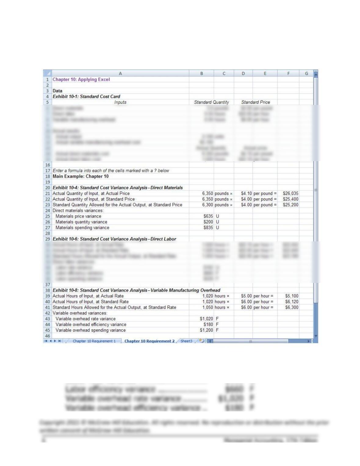
2. With the revised data, the worksheet should look like this:
Parts a, b, and c:
Materials price variance ………………….
$635
U
Materials quantity variance ……………..
$200
U
Labor efficiency variance ………………..
$660
F
Variable overhead rate variance ……….
F
The Foundational 15
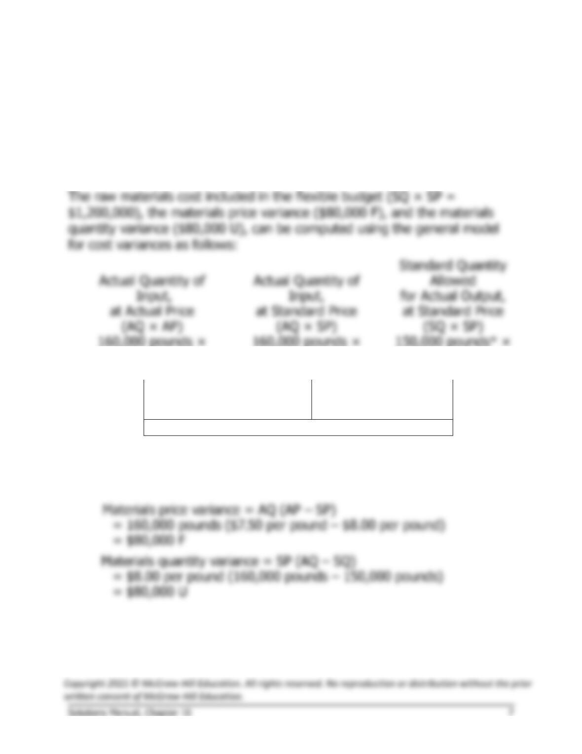
1. The raw materials cost included in the planning budget is $1,000,000
(= 25,000 pounds × 5 pounds per unit × $8.00 per pound =
$1,000,000).
2, 3, and 4.
$7.50 per pound
= $1,200,000
$8.00 per pound
= $1,280,000
$8.00 per pound
= $1,200,000
Materials price
variance = $80,000 F
Materials quantity
variance = $80,000 U
Spending variance = $0
*30,000 units × 5 pounds per unit = 150,000 pounds
Alternatively, the variances can be computed using the formulas:
The Foundational 15 (continued)
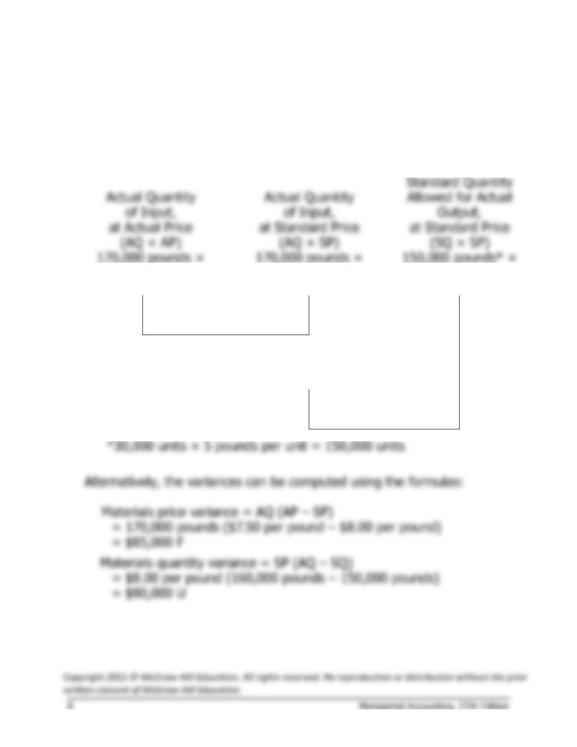
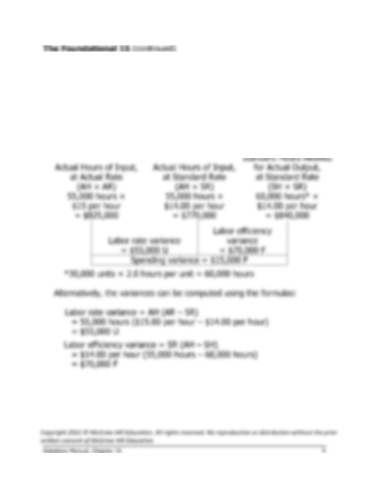
5. and 6.
The materials price variance ($85,000 F) and the materials quantity
variance ($80,000 U) can be computed as follows:
$7.50 per pound
= $1,275,000
$8.00 per pound
= $1,360,000
$8.00 per pound
= $1,200,000
Materials price variance
= $85,000 F
160,000 pounds ×
$8.00 per pound
= $1,280,000
Materials quantity
variance = $80,000 U
7. The direct labor cost included in the planning budget is $700,000 (=
25,000 units × 2 hours per unit × $14.00 per hour = $700,000).
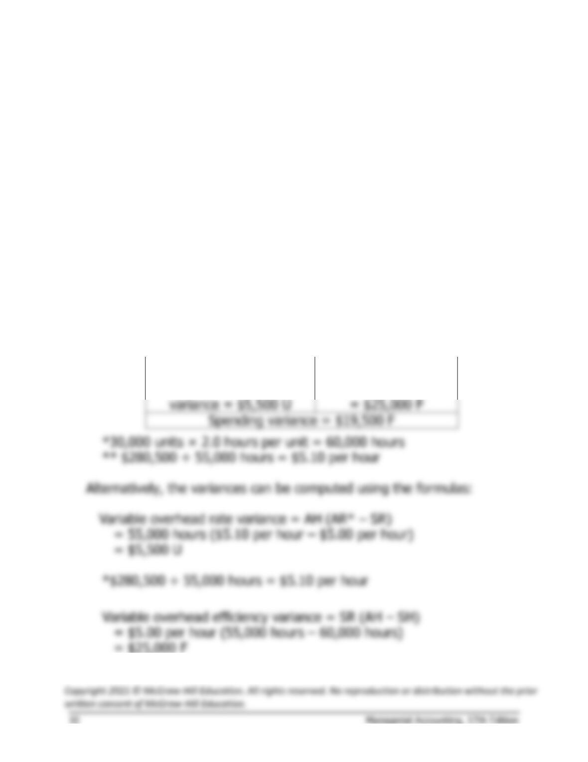
8, 9, 10, and 11.
The direct labor cost included in the flexible budget (SH × SR = $840,000),
the labor rate variance ($55,000 U), the labor efficiency variance ($70,000
F), and the labor spending variance ($15,000 F) can be computed using
the general model for cost variances as follows:
The Foundational 15 (continued)
12. The variable manufacturing overhead cost included in the planning
budget is $250,000 (= 50,000 hours × $5.00 per hour = $250,000).
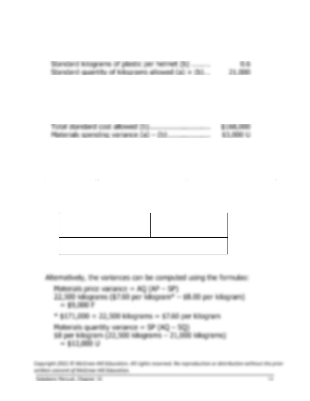
13, 14, and 15.
The variable overhead cost included in the flexible budget (SH × SR =
$300,000), the variable overhead rate variance ($5,500 U), and the
variable overhead efficiency variance ($25,000 F) can be computed using
the general model for cost variances as follows:
Actual Hours of Input,
at Actual Rate
(AH × AR)
Actual Hours of Input,
at Standard Rate
(AH × SR)
Standard Hours Allowed
for Actual Output,
at Standard Rate
(SH × SR)
55,000 hours ×
$5.10 per hour**
= $280,500
55,000 hours ×
$5.00 per hour
= $275,000
60,000 hours* ×
$5.00 per hour
= $300,000
Variable overhead rate
Variable overhead
efficiency variance
Exercise 10-1 (20 minutes)
1.
Number of helmets produced (a) ………………………
35,000
Standard kilograms of plastic per helmet (b) ……….
Standard quantity of kilograms allowed (a) × (b) ….
21,000
2.
Standard quantity of kilograms allowed (a) ………….
21,000
Standard cost per kilogram (b) …………………………
$8
Standard cost allowed for actual output (a) × (b) …
$168,000
3.
Actual cost incurred (given) (a) ………………………..
$171,000
Total standard cost allowed (b)…………………………
Materials spending variance (a) – (b) ………………..
$3,000 U
4.
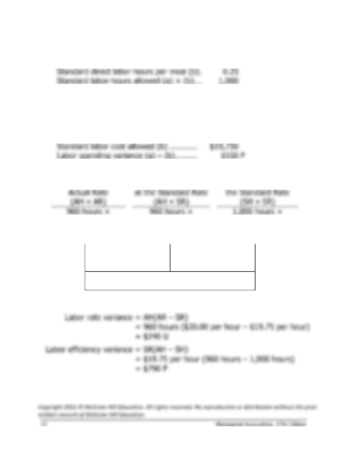
Actual Quantity
of Input, at
Actual Price
Actual Quantity of Input,
at Standard Price
Standard Quantity
Allowed for Output, at
Standard Price
(AQ × AP)
(AQ × SP)
(SQ × SP)
22,500 kilograms ×
21,000 kilograms* ×
$8 per kilogram
$8 per kilogram
$171,000
= $180,000
= $168,000
Materials price variance,
$9,000 F
Materials quantity
variance,
$12,000 U
Spending variance,
$3,000 U
*35,000 helmets × 0.6 kilograms per helmet = 21,000 kilograms
Exercise 10-2 (20 minutes)
1.
Number of meals prepared (a) …………….
4,000
Standard direct labor-hours per meal (b) .
Standard labor-hours allowed (a) × (b) …
2.
Standard labor-hours allowed (a) ………..
1,000
Standard direct labor cost per hour (b) ….
$19.75
Standard labor cost allowed (a) × (b) …..
$19,750
3.
Actual cost incurred (a) ……………………
$19,200
Standard labor cost allowed (b) …………
$19,750
Labor spending variance (a) – (b) ………
F
4.
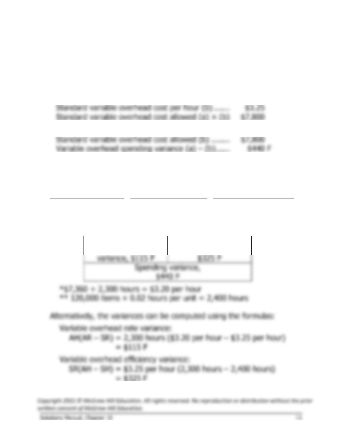
Actual Hours of
Input, at the
Actual Hours of Input,
Standard Hours
Allowed for Output, at
$20.00 per hour
$19.75 per hour
$19.75 per hour
= $19,200
= $18,960
= $19,750
Labor rate variance,
$240 U
Labor efficiency
variance,
$790 F
Spending variance,
$550 F
Alternatively, the variances can be computed using the formulas:
Exercise 10-3 (20 minutes)
1.
Number of items shipped (a) ………………………….
120,000
Standard labor-hours per item (b) ……………………
0.02
Standard quantity of labor-hours allowed (a) × (b)
2,400
2.
Standard quantity of labor-hours allowed (a) ……..
2,400
Standard variable overhead cost per hour (b) …….
Standard variable overhead cost allowed (a) × (b)
3.
Actual variable overhead cost incurred (a) …………
$7,360
Standard variable overhead cost allowed (b) ……..
Variable overhead spending variance (a) – (b) ……
F
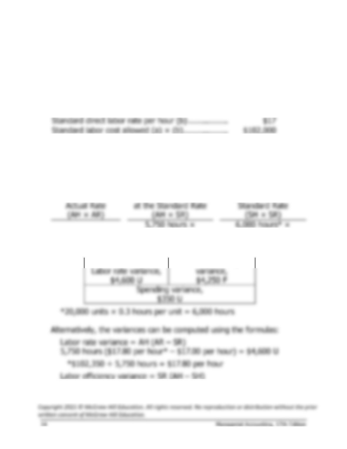
4.
Actual Hours of
Input, at the
Actual Rate
Actual Hours of Input,
at the Standard Rate
Standard Hours
Allowed for Output, at
the Standard Rate
(AH × AR)
(AH × SR)
(SH × SR)
2,300 hours ×
$3.20 per hour*
2,300 hours ×
$3.25 per hour
2,400 hours** ×
$3.25 per hour
= $7,360
= $7,475
= $7,800
Variable overhead rate
Variable overhead
efficiency variance,
Exercise 10-4 (30 minutes)
1.
Number of units manufactured (a) …………………..
20,000
Standard labor time per unit
(18 minutes ÷ 60 minutes per hour) (b) …………
0.3
Standard labor-hours allowed (a) × (b) …………….
6,000
2.
Standard labor-hours allowed (a)
6,000
Standard direct labor rate per hour (b) ……………..
Standard labor cost allowed (a) × (b) ……………….
3.
Actual direct labor cost (a) ……………………………..
$102,350
Standard labor cost allowed (b) ………………………
$102,000
Labor spending variance (a) – (b) ……………………
$350 U
4.
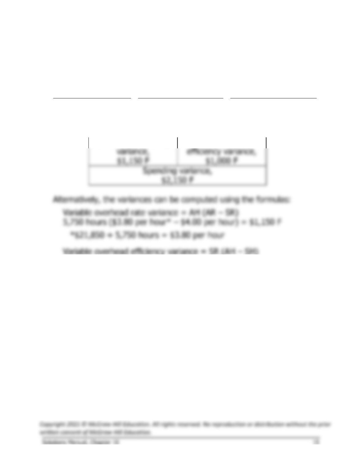
Actual Hours of
Input, at the
Actual Hours of Input,
Standard Hours Allowed
for Output, at the
$17.00 per hour
$17.00 per hour
$102,350
= $97,750
= $102,000
Labor efficiency
$17.00 per hour (5,750 hours – 6,000 hours) = $4,250 F
Exercise 10-4 (continued)
5.
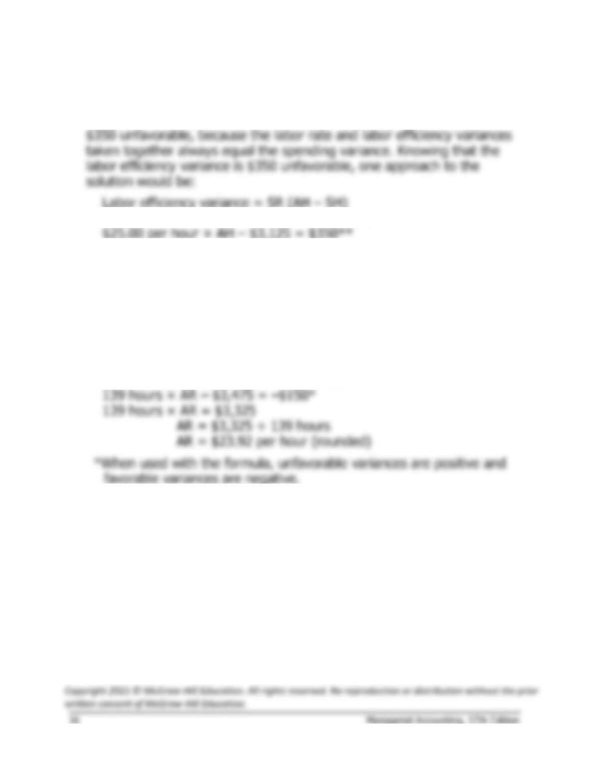
Actual Hours of
Input, at the
Actual Rate
Actual Hours of Input,
at the Standard Rate
Standard Hours
Allowed for Output, at
the Standard Rate
(AH × AR)
(AH × SR)
(SH × SR)
5,750 hours ×
$4.00 per hour
6,000 hours ×
$4.00 per hour
$21,850
= $23,000
= $24,000
Variable overhead rate
Variable overhead
$4.00 per hour (5,750 hours – 6,000 hours) = $1,000 F
Exercise 10-5 (20 minutes)
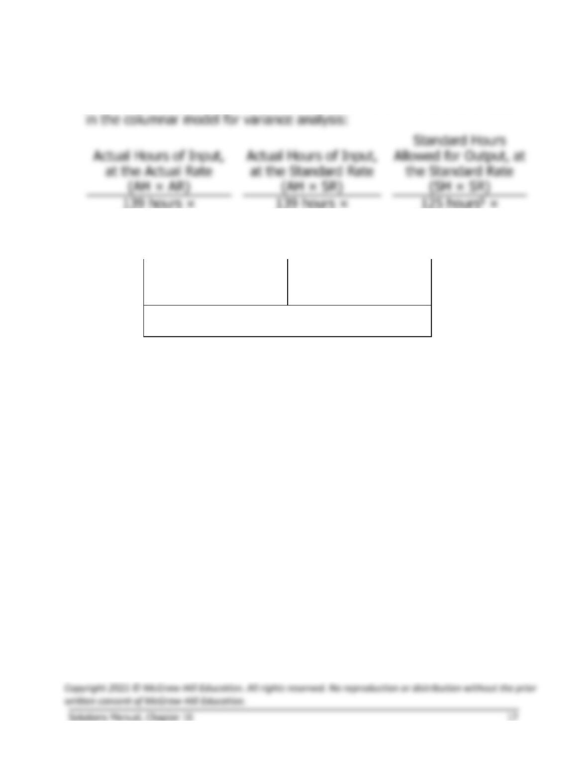
1. If the labor spending variance is $200 unfavorable, and the labor rate
variance is $150 favorable, then the labor efficiency variance must be
$25.00 per hour (AH – 125 hours*) = $350 U
$25.00 per hour × AH = $3,475
AH = $3,475 ÷ $25.00 per hour
AH = 139 hours
*
50 jobs × 2.5 hours per job = 125 hours
**
When used with the formula, unfavorable variances are positive and
favorable variances are negative.
2. Labor rate variance = AH (AR – SR)
139 hours (AR – $25.00 per hour) = $150 F
Exercise 10-5 (continued)
An alternative approach would be to work from known to unknown data
$23.92 per hour
$25.00 per hour*
$25.00 per hour*
= $3,325
= $3,475
= $3,125
Labor rate variance,
$150 F*
Labor efficiency
variance,
$350 U
Spending variance,
$200 U*
§50 tune-ups* × 2.5 hours per tune-up* = 125 hours
*Given
Exercise 10-6 (20 minutes)
1.
Actual Quantity
of Input, at
Actual Price
Actual Quantity
of Input, at
Standard Price
Standard Quantity
Allowed for Output,
at Standard Price
(AQ × AP)
(AQ × SP)
(SQ × SP)
20,000 pounds ×
$2.35 per pound
20,000 pounds ×
$2.50 per pound
18,400 pounds* ×
$2.50 per pound
= $47,000
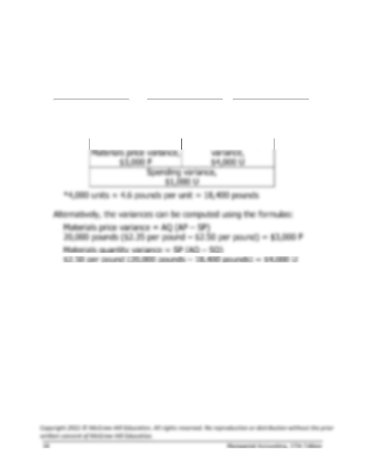
= $50,000
= $46,000
Materials quantity