10-21
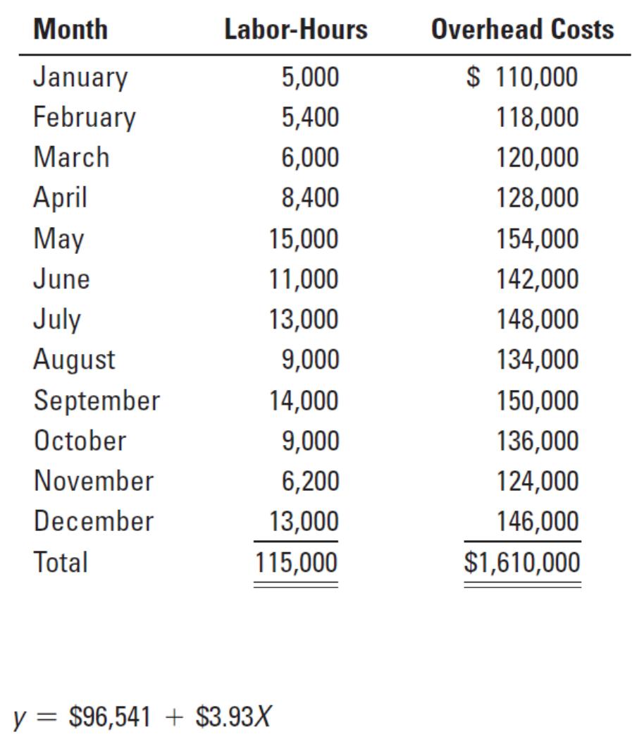
Baiman has recently become aware of regression analysis. He estimated the following regression
equation with overhead costs as the dependent variable and labor-hours as the independent
variable:
Required:
1. Plot the relationship between overhead costs and labor-hours. Draw the regression line and
evaluate it using the criteria of economic plausibility, goodness of fit, and slope of the
regression line.
2. Using data from the regression analysis, what is the variable cost per person for a standard
party?
10-22
3. Stan Baiman has been asked to prepare a bid for a 200-person standard party to be given next
month. Determine the minimum bid price that Baiman would be willing to submit to recoup
variable costs.
SOLUTION
10-23
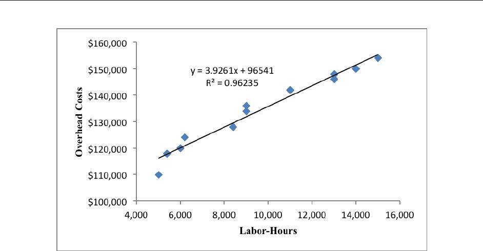
SOLUTION EXHIBIT 10-26
Regression Line of Overhead Costs on Labor-Hours for Stan Baiman’s Catering Company
10-24
10-27 High-low, regression
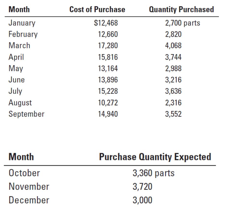
Mandy Knox is the new manager of the materials storeroom for Timken Manufacturing. Mandy
has been asked to estimate future monthly purchase costs for part #696, used in two of Timken’s
products. Mandy has purchase cost and quantity data for the past 9 months as follows:
Estimated monthly purchases for this part based on expected demand of the two products for the
rest of the year are as follows:
Required:
1. The computer in Mandy’s office is down, and Mandy has been asked to immediately provide
an equation to estimate the future purchase cost for part #696. Mandy grabs a calculator and
uses the high- low method to estimate a cost equation. What equation does she get?
2. Using the equation from requirement 1, calculate the future expected purchase costs for each
of the last 3 months of the year.
10-25
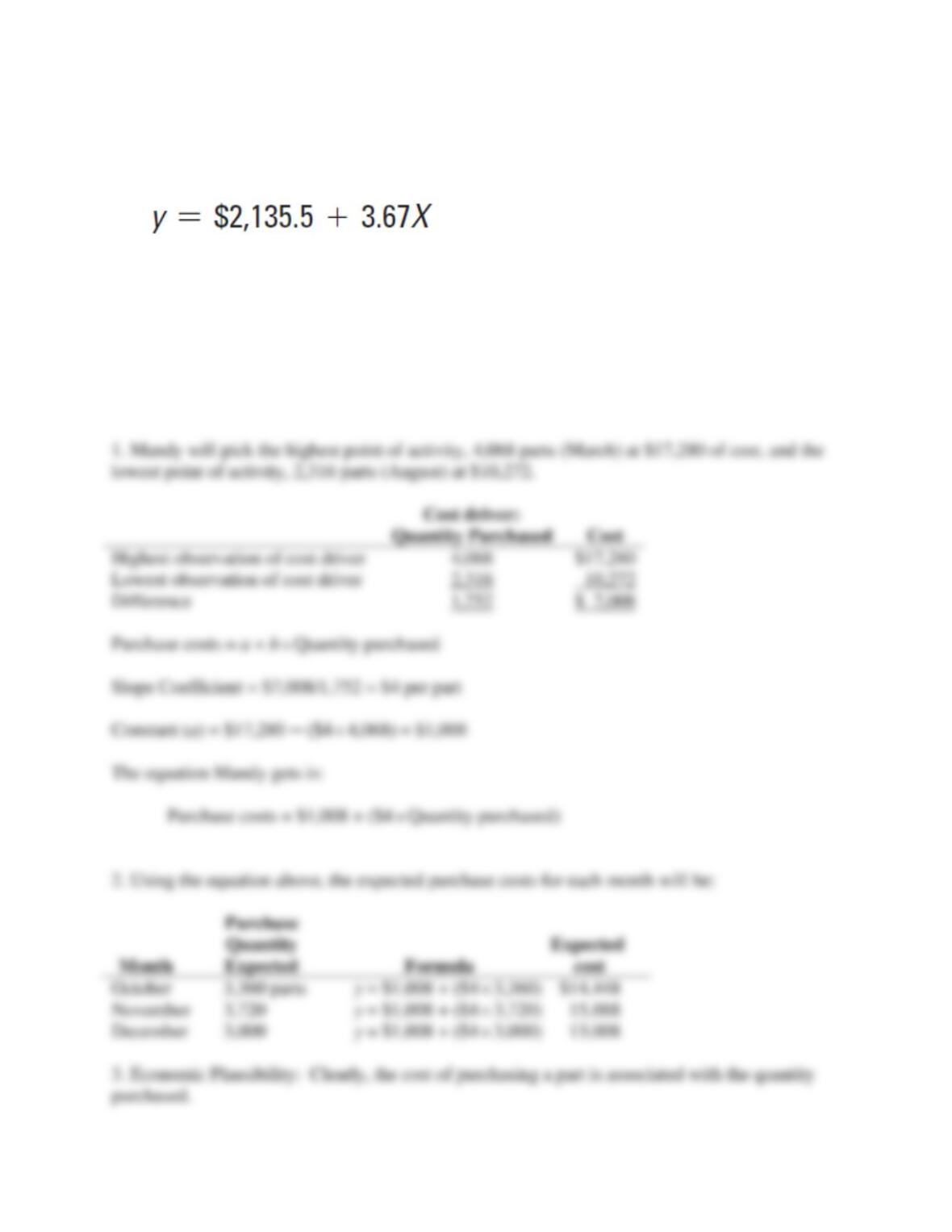
3. After a few hours Mandy’s computer is fixed. Mandy uses the first 9 months of data and
regression analysis to estimate the relationship between the quantity purchased and purchase
costs of part #696. The regression line Mandy obtains is as follows:
Evaluate the regression line using the criteria of economic plausibility, goodness of fit, and
significance of the independent variable. Compare the regression equation to the equation
based on the high-low method. Which is a better fit? Why?
4. Use the regression results to calculate the expected purchase costs for October, November,
and December. Compare the expected purchase costs to the expected purchase costs
calculated using the high-low method in requirement 2. Comment on your results.
SOLUTION
10-26
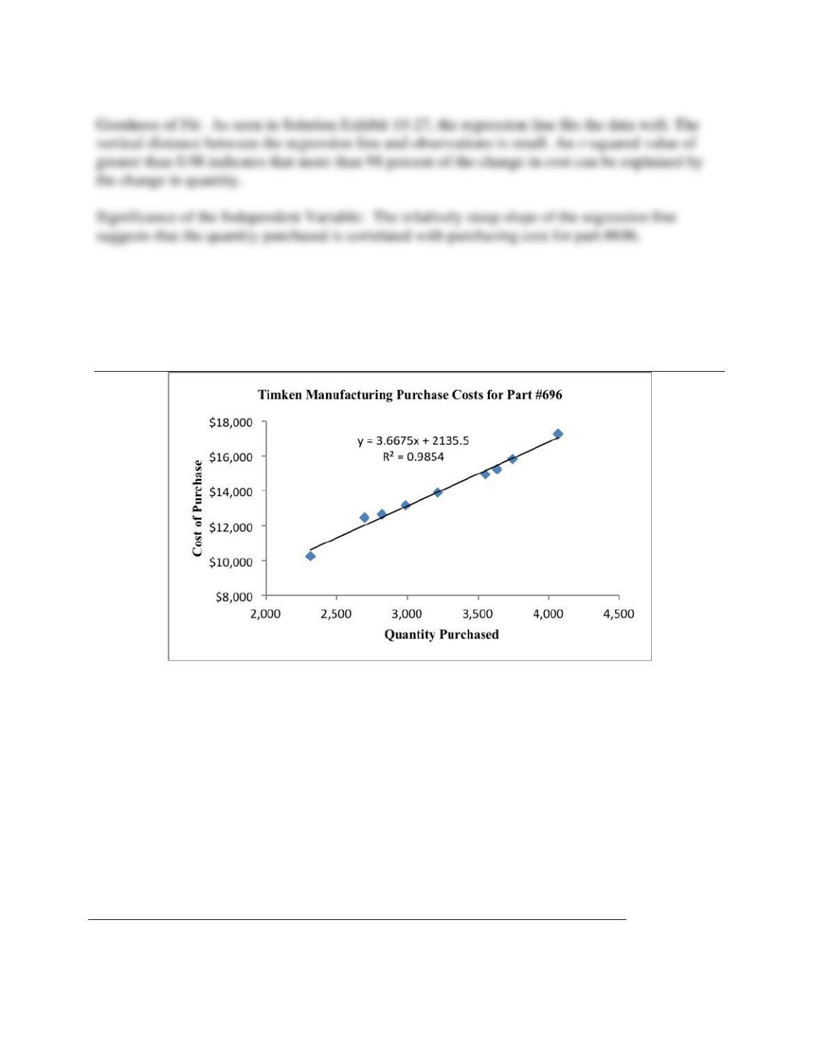
SOLUTION EXHIBIT 10-27
According to the regression, Mandy’s original estimate of fixed cost is too low given all the data
points. The original slope is too steep but only by 33 cents. So, the variable rate is lower, but the
fixed cost is higher for the regression line than for the high-low cost equation.
The regression is the more accurate estimate because it uses all available data (all nine data
points), while the high-low method only relies on two data points and may therefore miss some
important information contained in the other data.
4. Using the regression equation, the purchase costs for each month will be:
Month
Purchase
Quantity
Expected
Formula
Expected cost
October 3,360 parts y = $2,135.50 + ($3.67
3,360) $14,466.70
November 3,720 y = $2,135.50 + ($3.67
3,720) 15,787.90
10-27
December 3,000 y = $2,135.50 + ($3.67
3,000) 13,145.50
Although the two equations are different in both fixed element and variable rate, within the
relevant range they give similar expected costs. This implies that the high and low points of the
data are a reasonable representation of the total set of points within the relevant range.
10-28 (20 min.) Learning curve, cumulative average-time learning model.
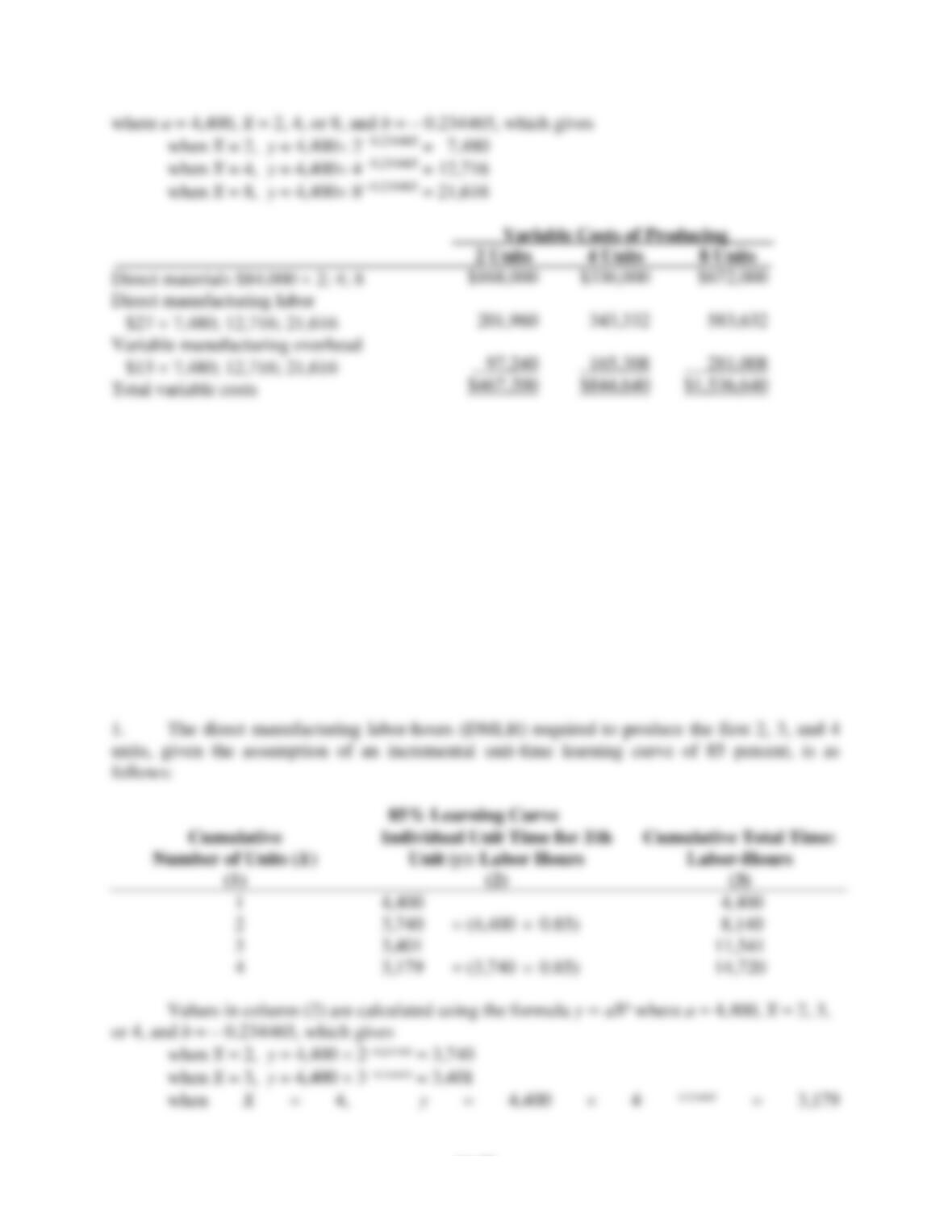
Northern Defense manufactures radar systems. It has just completed the manufacture of its first
newly designed system, RS-32. Manufacturing data for the RS-32 follow:
Required:
Calculate the total variable costs of producing 2, 4, and 8 units.
SOLUTION
10-28
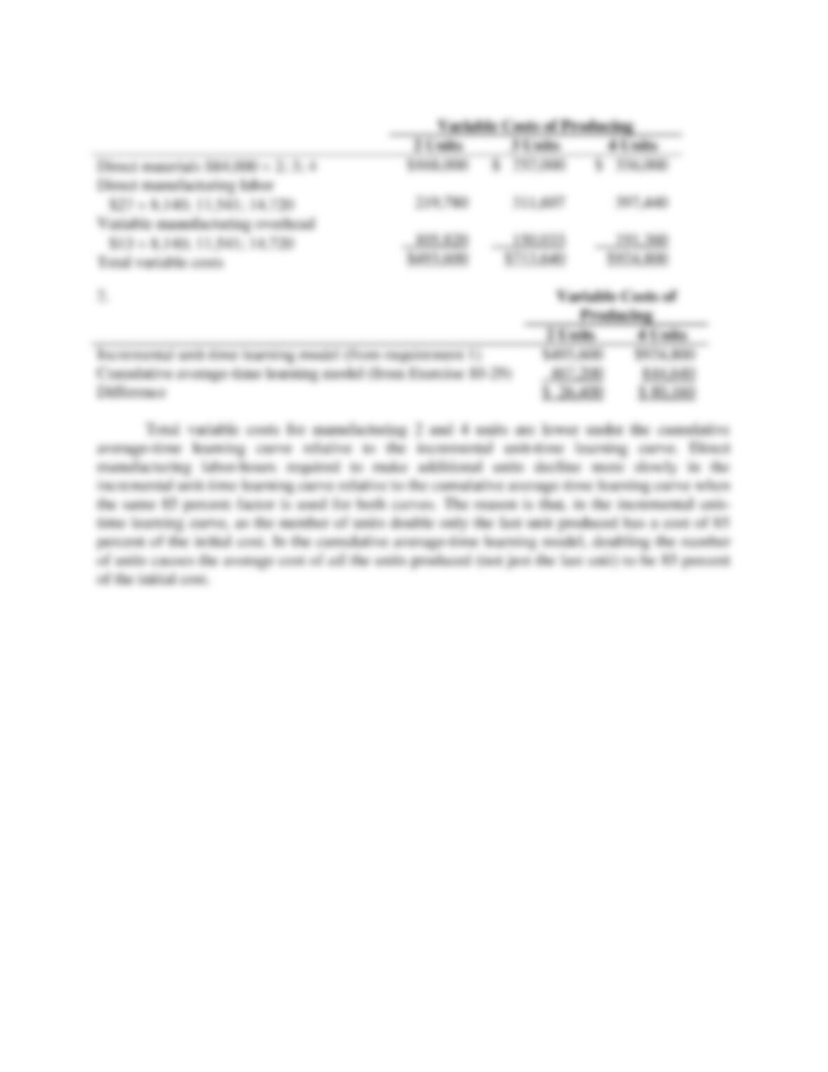
10-29 (20 min.) Learning curve, incremental unit-time learning model.
Assume the same information for Northern Defense as in Exercise 10-28, except that Northern
Defense uses an 85% incremental unit-time learning model as a basis for predicting direct
manufacturing labor-hours. (An 85% learning curve means b = -0.234465.)
Required:
1. Calculate the total variable costs of producing 2, 3, and 4 units.
2. If you solved Exercise 10-28, compare your cost predictions in the two exercises for 2 and 4
units. Why are the predictions different? How should Northern Defense decide which model
it should use?
SOLUTION
10-29
10-30 (25 min.) High-low method.
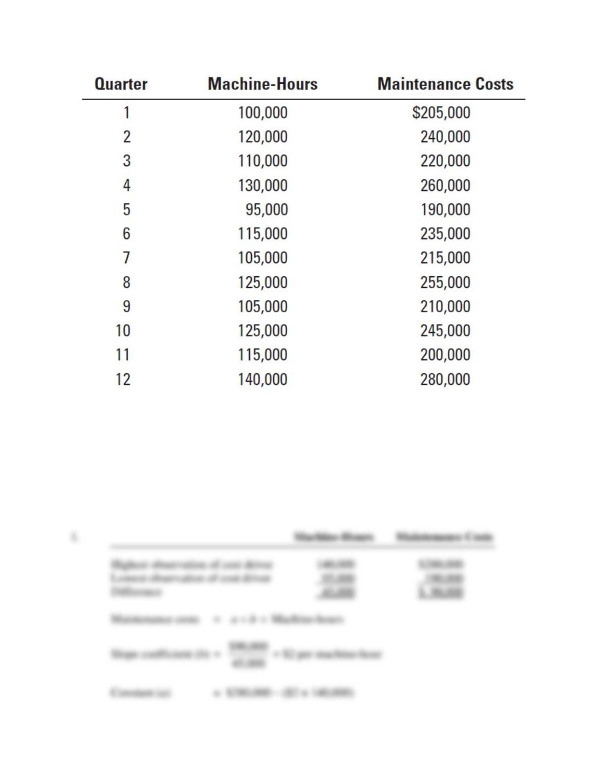
Ken Howard, financial analyst at KMW Corporation, is examining the behavior of quarterly
maintenance costs for budgeting purposes. Howard collects the following data on machine–
hours worked and maintenance costs for the past 12 quarters:
10-30
Required:
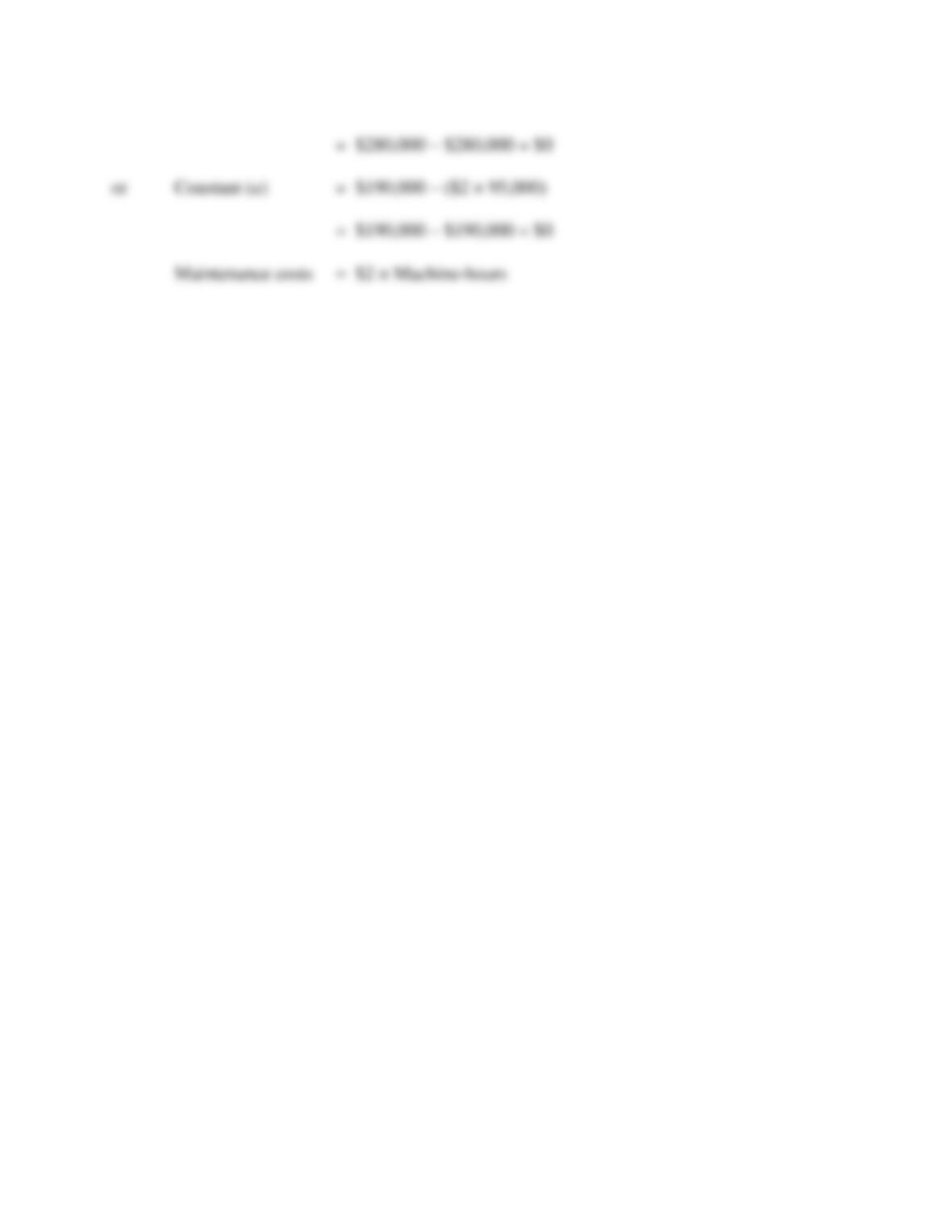
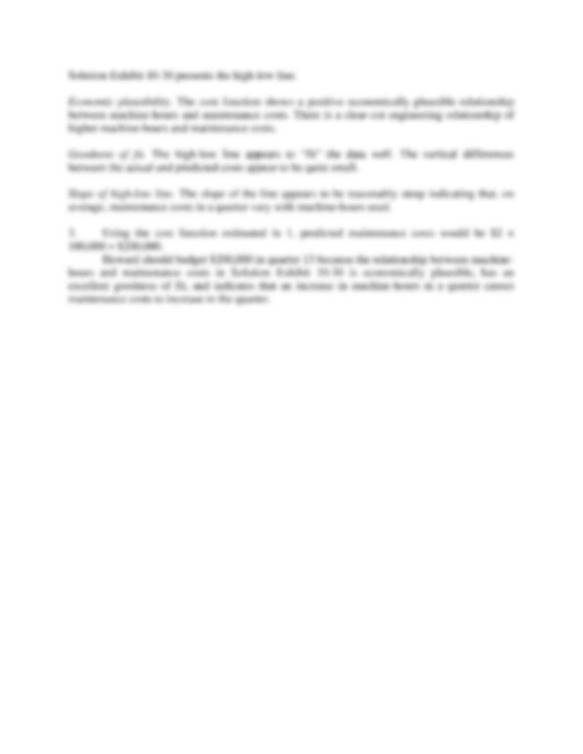
1. Estimate the cost function for the quarterly data using the high-low method.
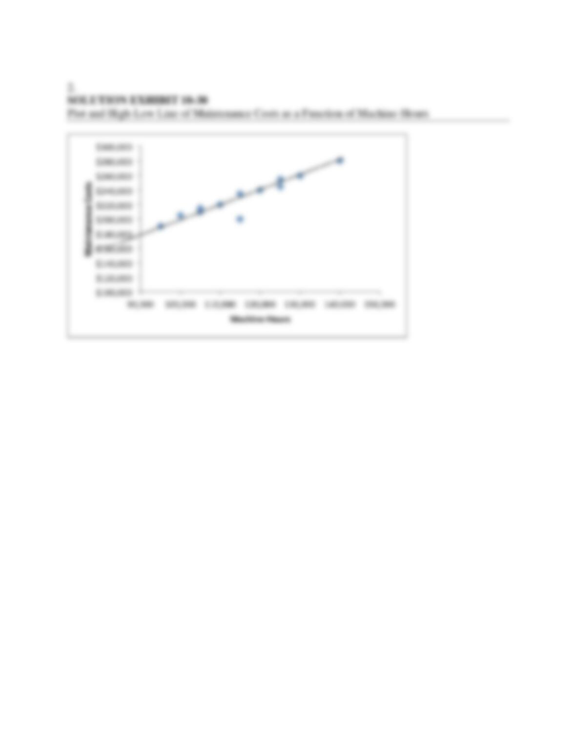
2. Plot and comment on the estimated cost function.
3. Howard anticipates that KMW will operate machines for 100,000 hours in quarter 13.
Calculate the predicted maintenance costs in quarter 13 using the cost function estimated in
requirement 1.
SOLUTION
10-31
10-32
10-33
10-31 (30min.) High-low method and regression analysis.
Fresh Choice, a cooperative of organic family-owned farms outside of Madison, Wisconsin, has
recently started a fresh produce club to provide support to the group’s member farms and to
promote the benefits of eating organic, locally produced food to the nearby suburban community.
Families pay a seasonal membership fee of $75 and place their orders a week in advance for a
price of $35 per order. In turn, Fresh Choice delivers fresh-picked seasonal local produce to
several neighborhood distribution points. Seven hundred families joined the club for the first
season, but the number of orders varied from week to week.
Daniel Craig has run the produce club for the first 10-week season. Before becoming a
farmer, Daniel had been a business major in college, and he remembers a few things about cost
analysis. In planning for next year, he wants to know how many orders will be needed each week
for the club to break even, but first he must estimate the club’s fixed and variable costs. He has
collected the following data over the club’s first 10 weeks of operation:
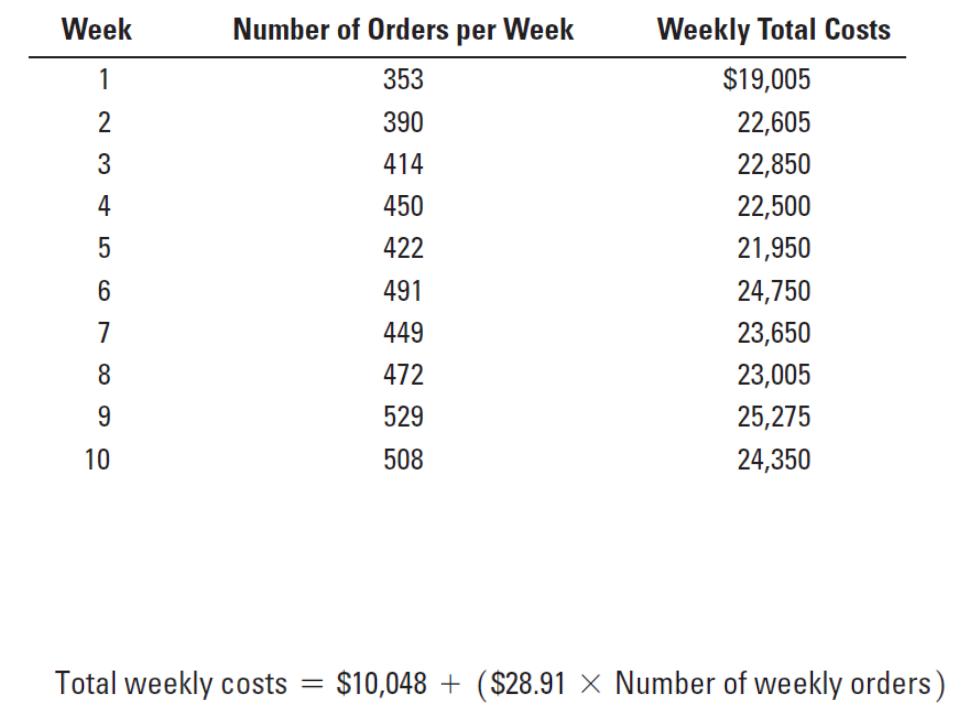
10-34
Required:
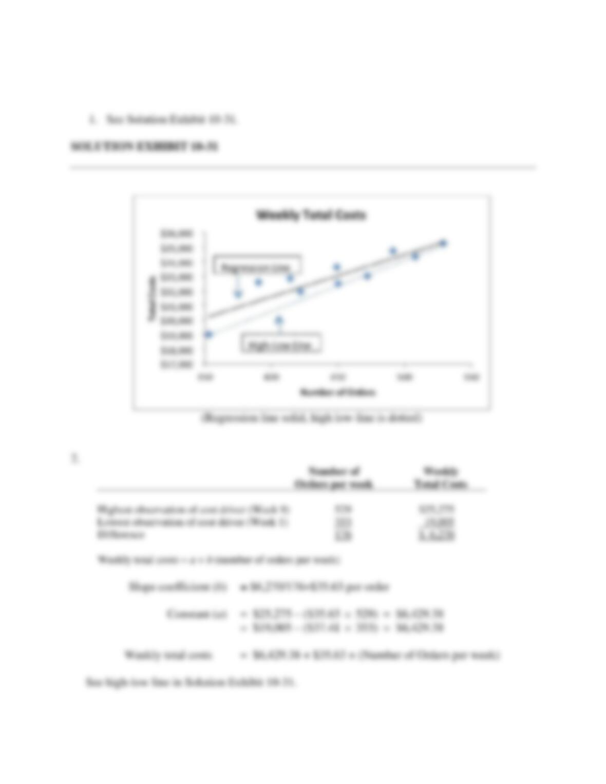
1. Plot the relationship between number of orders per week and weekly total costs.
2. Estimate the cost equation using the high-low method, and draw this line on your graph.
3. Harvey uses his computer to calculate the following regression formula:
Draw the regression line on your graph. Use your graph to evaluate the regression line using
the criteria of economic plausibility, goodness of fit, and significance of the independent
variable. Is the cost function estimated using the high-low method a close approximation of
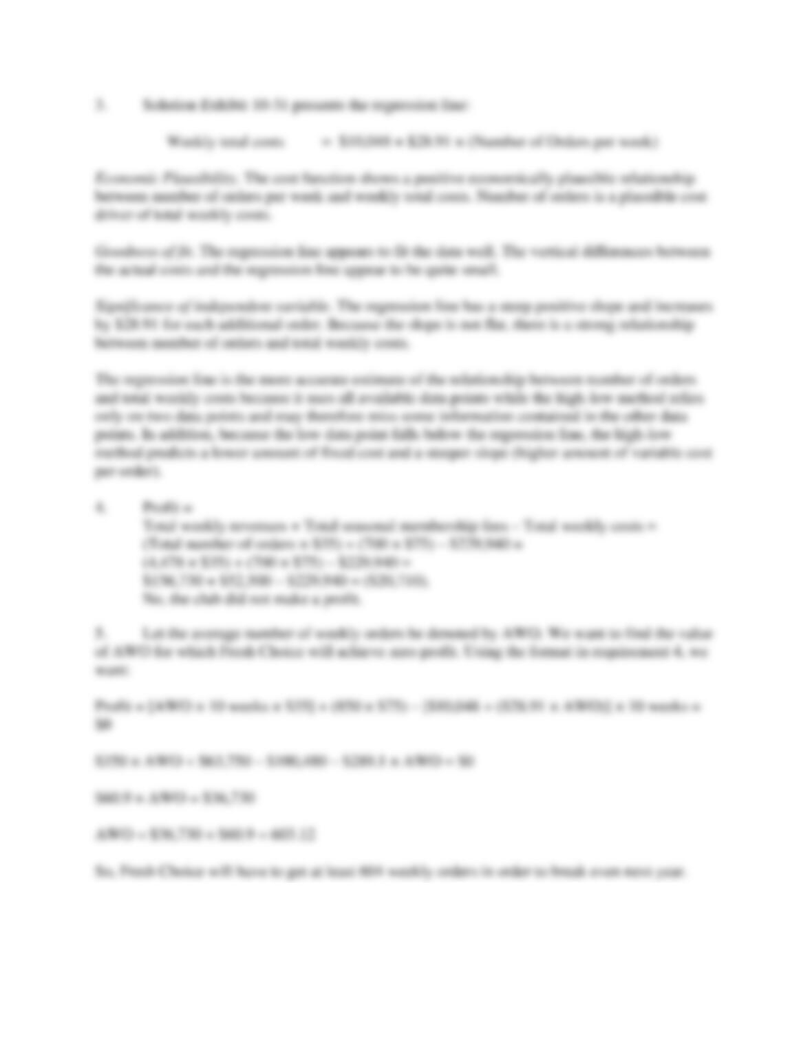
the cost function estimated using the regression method? Explain briefly.
4. Did Fresh Choice break even this season? Remember that each of the families paid a
seasonal membership fee of $75.
5. Assume that 850 families join the club next year and that prices and costs do not change.
How many orders, on average, must Fresh Choice receive each week to break even?
10-35
SOLUTION
10-36
10-32 (30−40 min.) High-low method, regression analysis.
10-37
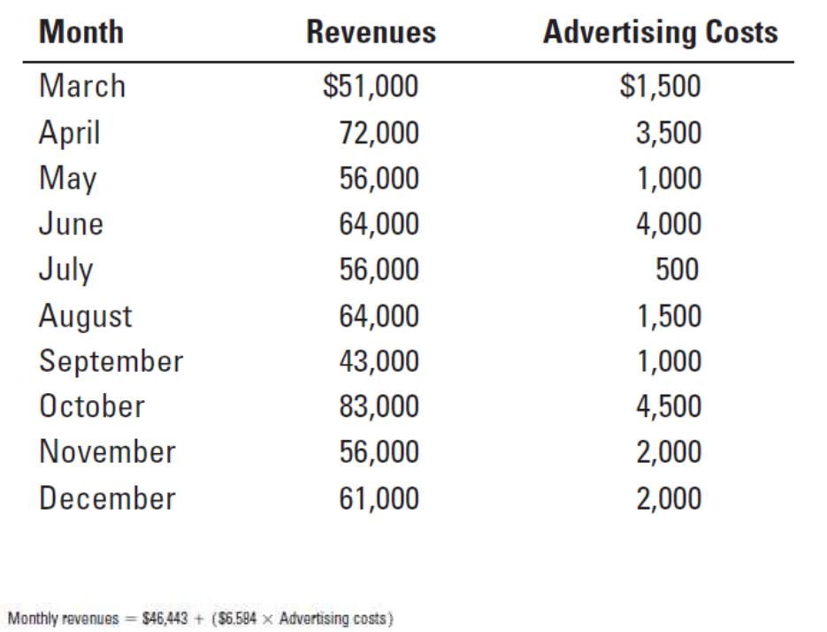
(CIMA, adapted) Anna Schaub, the financial manager at the Mangiamo restaurant, is checking to
see if there is any relationship between newspaper advertising and sales revenues at the
restaurant. She obtains the following data for the past 10 months:
She estimates the following regression equation:
Required:
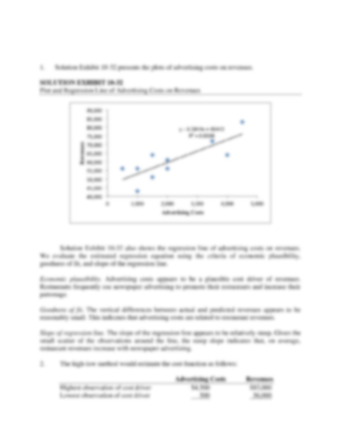
1. Plot the relationship between advertising costs and revenues. Also draw the regression line
and evaluate it using the criteria of economic plausibility, goodness of fit, and slope of the
regression line.
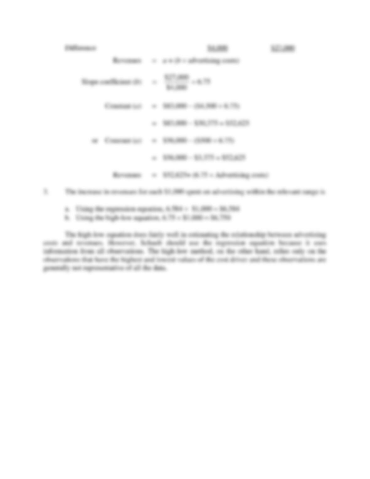
2. Use the high-low method to compute the function relating advertising costs and revenues.
3. Using (a) the regression equation and (b) the high-low equation, what is the increase in
revenues for each $1,000 spent on advertising within the relevant range? Which method
should Schaub use to predict the effect of advertising costs on revenues? Explain briefly.
10-38
SOLUTION
10-39
10-40
10-33 (30 min.) Regression, activity-based costing, choosing cost drivers.
Parker Manufacturing has been using activity-based costing to determine the cost of product X–
678. One of the activities, “Inspection,” occurs just before the product is finished. Fitzgerald
inspects every 10th unit and has been using “number of units inspected” as the cost driver for
inspection costs. A significant component of inspection costs is the cost of the test kit used in
each inspection.
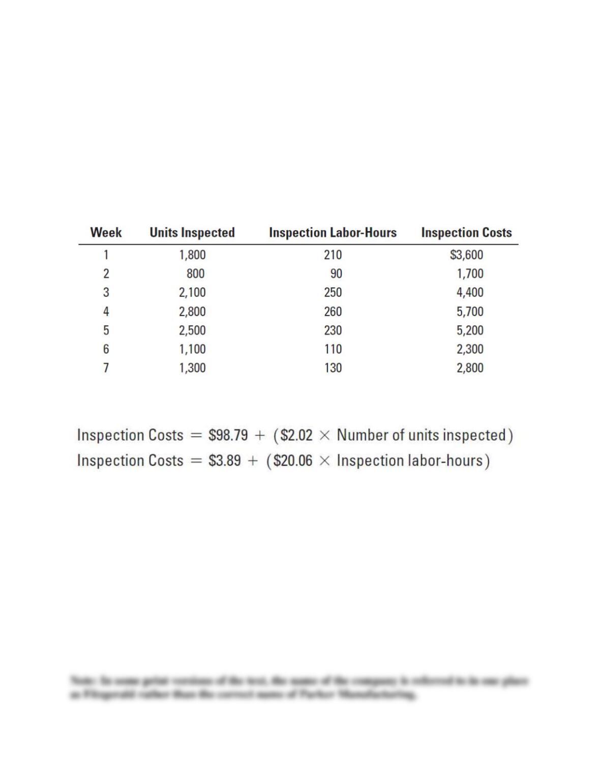
Sharon MacPhen, the line manager, is wondering if inspection labor-hours might be a better
cost driver for inspection costs. Sharon gathers information for weekly inspection costs, units
inspected, and inspection labor-hours as follows:
Sharon runs regressions on each of the possible cost drivers and estimates these cost functions:
Required:
1. Explain why number of units inspected and inspection labor-hours are plausible cost drivers
of inspection costs.
2. Plot the data and regression line for units inspected and inspection costs. Plot the data and
regression line for inspection labor-hours and inspection costs. Which cost driver of
inspection costs would you choose? Explain.
3. Sharon expects inspectors to work 160 hours next period and to inspect 1,500 units. Using
the cost driver you chose in requirement 2, what amount of inspection costs should Sharon
budget? Explain any implications of Sharon choosing the cost driver you did not choose in
requirement 2 to budget inspection costs.
SOLUTION