10-61
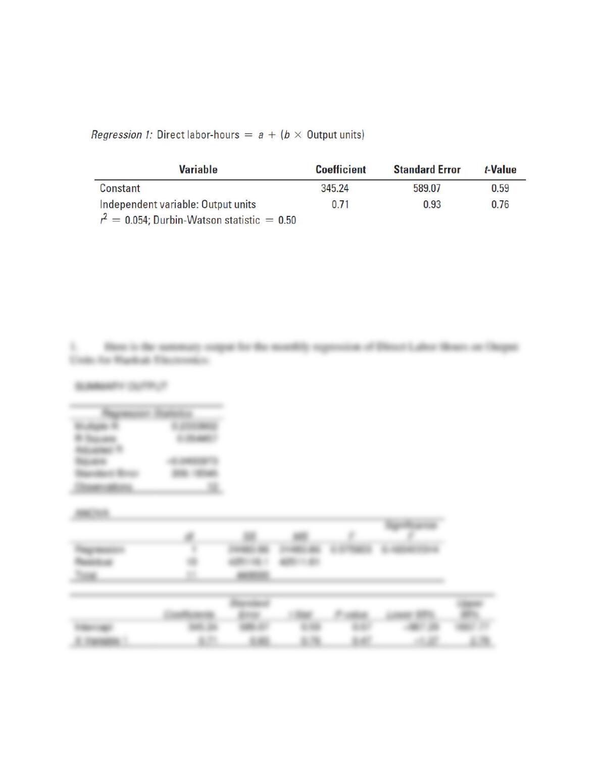
1. Inbee is keen to examine the relationship between direct labor consumption and output
levels. She decides to estimate this relationship using a simple linear regression based on the
monthly data. Verify that the following is the result obtained by Inbee:
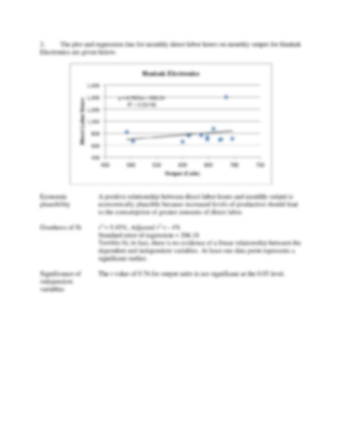
2. Plot the data and regression line for the above estimation. Evaluate the regression using the
criteria of economic plausibility, goodness of fit, and slope of the regression line.
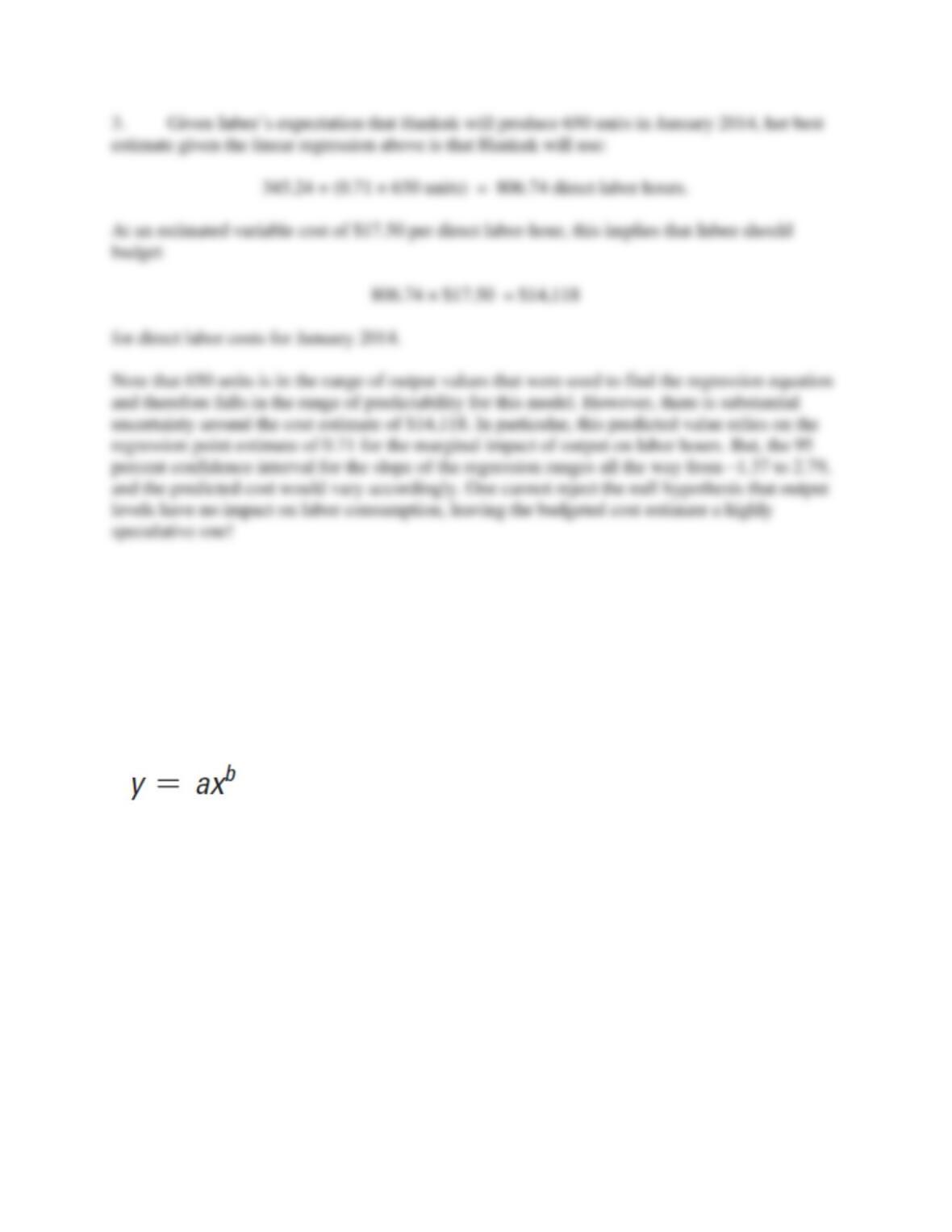
3. Inbee estimates that Hankuk has a variable cost of $17.50 per direct labor-hour. She expects
that Hankuk will produce 650 units in the next month, January 2014. What should she budget
as the expected variable cost? How confident is she of her estimate?
SOLUTION
10-62
10-63
10-40 (30 min.) Cost estimation, learning curves (continuation of 10-39).
Inbee is concerned that she still does not understand the relationship between output and labor
consumption. She consults with Jim Park, the head of engineering, and shares the results of her
regression estimation. Jim indicates that the production of new smartphone models exhibits
significant learning effects—as Hankuk gains experience with production, it can produce
additional units using less time. He suggests that it is more appropriate to specify the following
relationship:
where x is cumulative production in units, y is the cumulative average direct labor-hours per unit
(i.e., cumulative DLH divided by cumulative production), and a and b are parameters of the
learning effect.
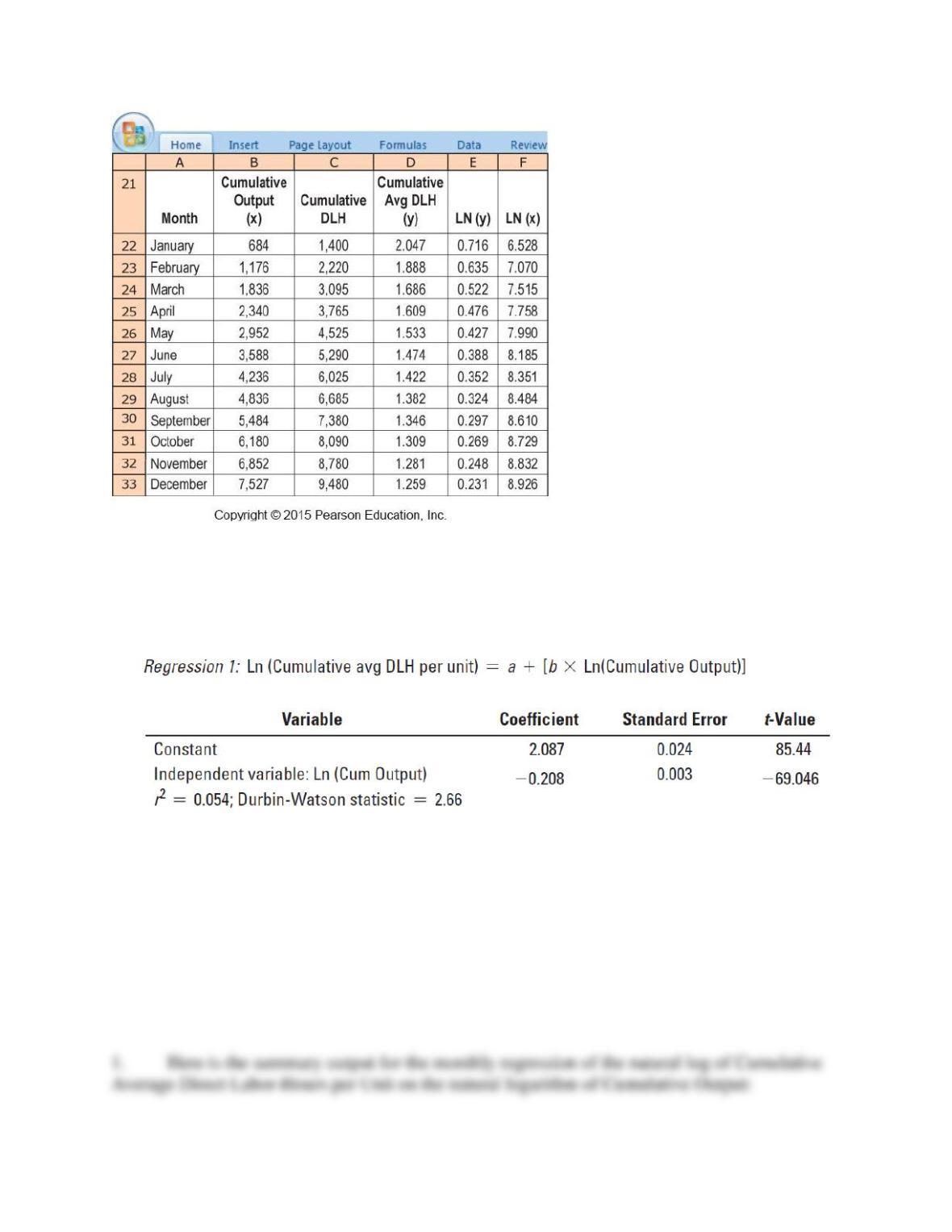
To estimate this, Inbee and Jim use the original data to calculate the cumulative output and
cumulative average labor-hours per unit for each month. They then take natural logarithms of
these variables in order to be able to estimate a regression equation. Here is the transformed data:
10-64
Required:
1. Estimate the relationship between the cumulative average direct labor-hours per unit and
cumulative output (both in logarithms). Verify that the following is the result obtained by
Inbee and Jim:
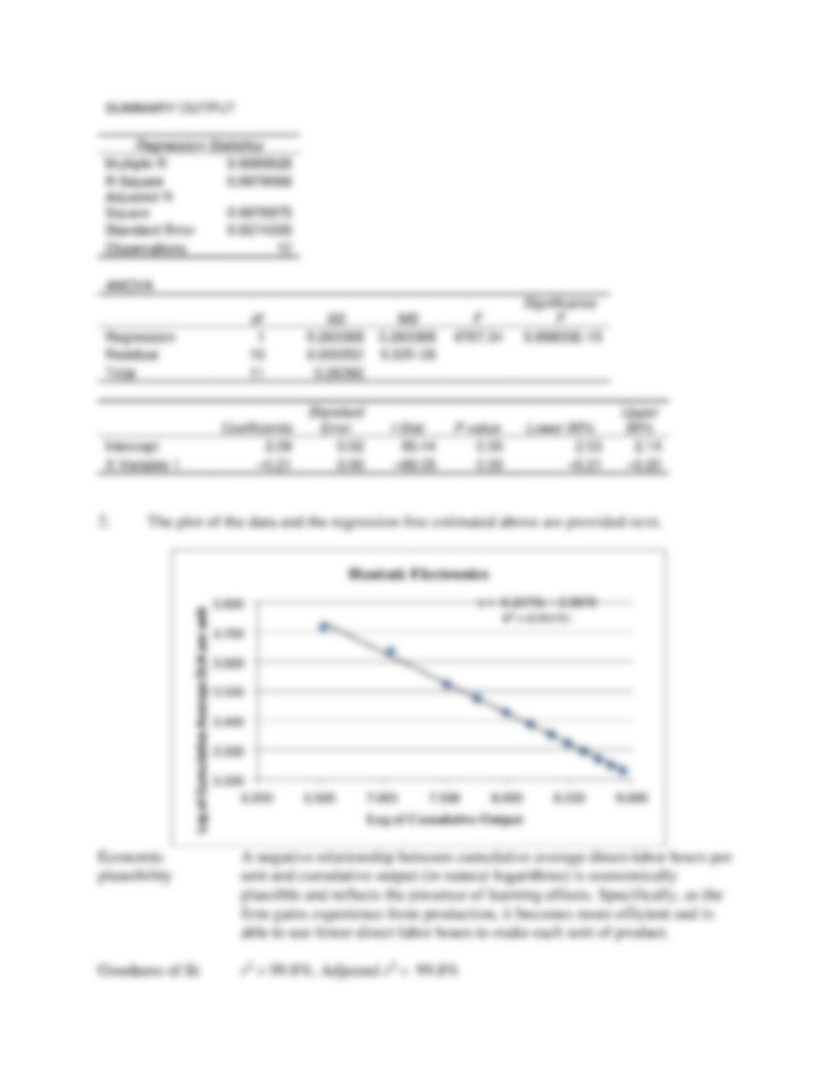
2. Plot the data and regression line for the above estimation. Evaluate the regression using the
criteria of economic plausibility, goodness of fit, and slope of the regression line.
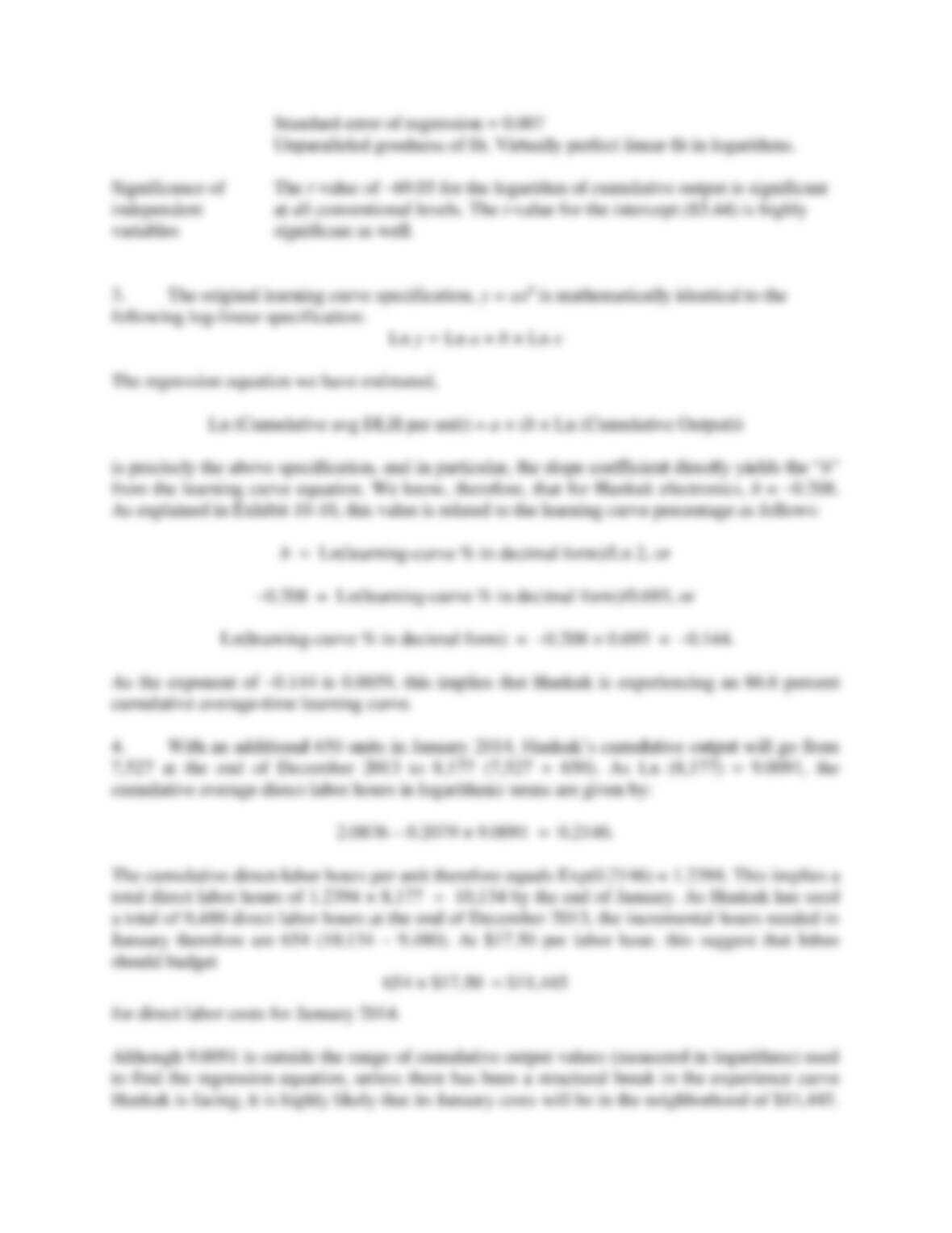
3. Verify that the estimated slope coefficient corresponds to an 86.6% cumulative average-time
learning curve.
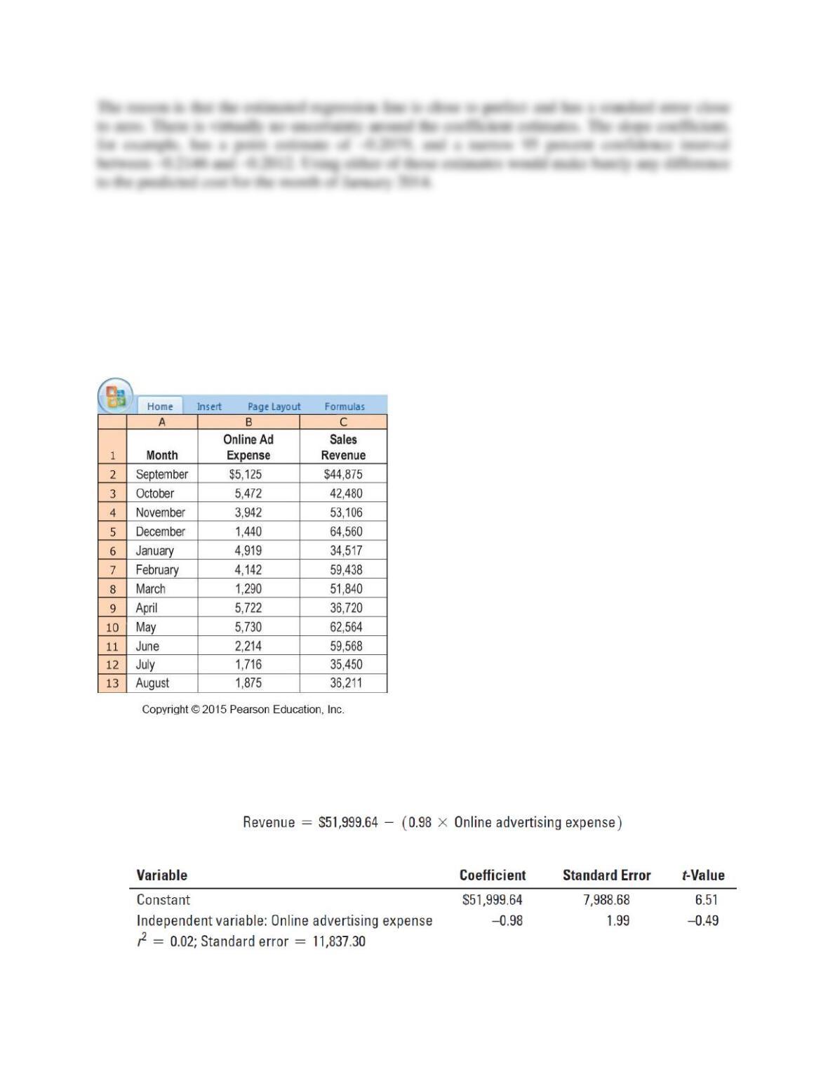
4. Based on this new estimation, how will Inbee revise her budget for Hankuk’s variable cost
for the expected output of 650 units in January 2014? How confident is she of this new cost
estimate?
SOLUTION
10-65
10-66
10-67
10-41 (25 min.) Interpreting regression results, matching time periods.
Nandita Summers works at Modus, a store that caters to fashion for young adults. Nandita is
responsible for the store’s online advertising and promotion budget. For the past year, she has
studied search engine optimization and has been purchasing keywords and display advertising on
Google, Facebook, and Twitter. In order to analyze the effectiveness of her efforts and to decide
whether to continue online advertising or move her advertising dollars back to traditional print
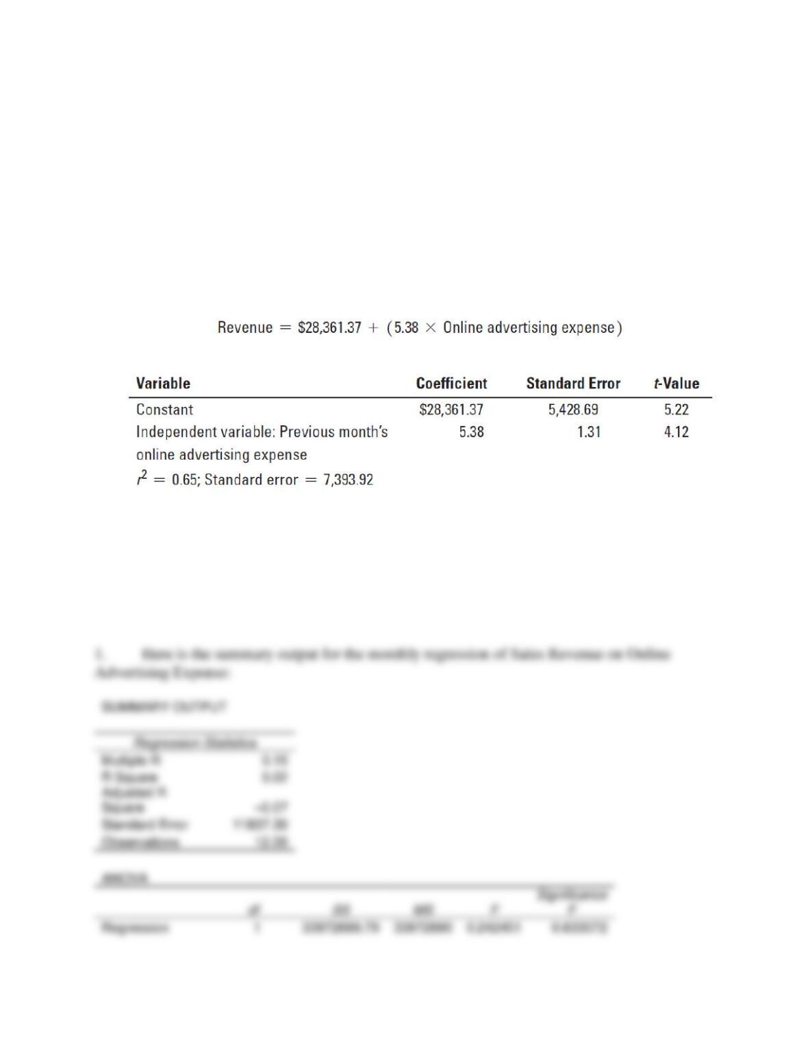
media, Nandita collects the following data:
Required:
1. Nandita performs a regression analysis, comparing each month’s online advertising expense
with that month’s revenue. Verify that she obtains the following result:
10-68
2. Plot the preceding data on a graph and draw the regression line. What does the cost formula
indicate about the relationship between monthly online advertising expense and monthly
revenues? Is the relationship economically plausible?
3. After further thought, Nandita realizes there may have been a flaw in her approach. In
particular, there may be a lag between the time customers click through to the Modus website
and peruse its social media content (which is when the online ad expense is incurred) and the
time they actually shop in the physical store. Nandita modifies her analysis by comparing
each month’s sales revenue to the advertising expense in the prior month. After discarding
September revenue and August advertising expense, show that the modified regression yields
the following:
4. What does the revised formula indicate? Plot the revised data on a graph. Is this relationship
economically plausible?
5. Can Nandita conclude that there is a cause-and-effect relationship between online advertising
expense and sales revenue? Why or why not?
SOLUTION

10-69
10-70
Coefficients
Standard
Error
t Stat
P-value
Lower 95%
Upper
95%
Intercept
51999.64
7988.68
6.51
0.00
34199.74
69799.54
X Variable 1
–0.98
1.99
–0.49
0.63
–5.41
3.45
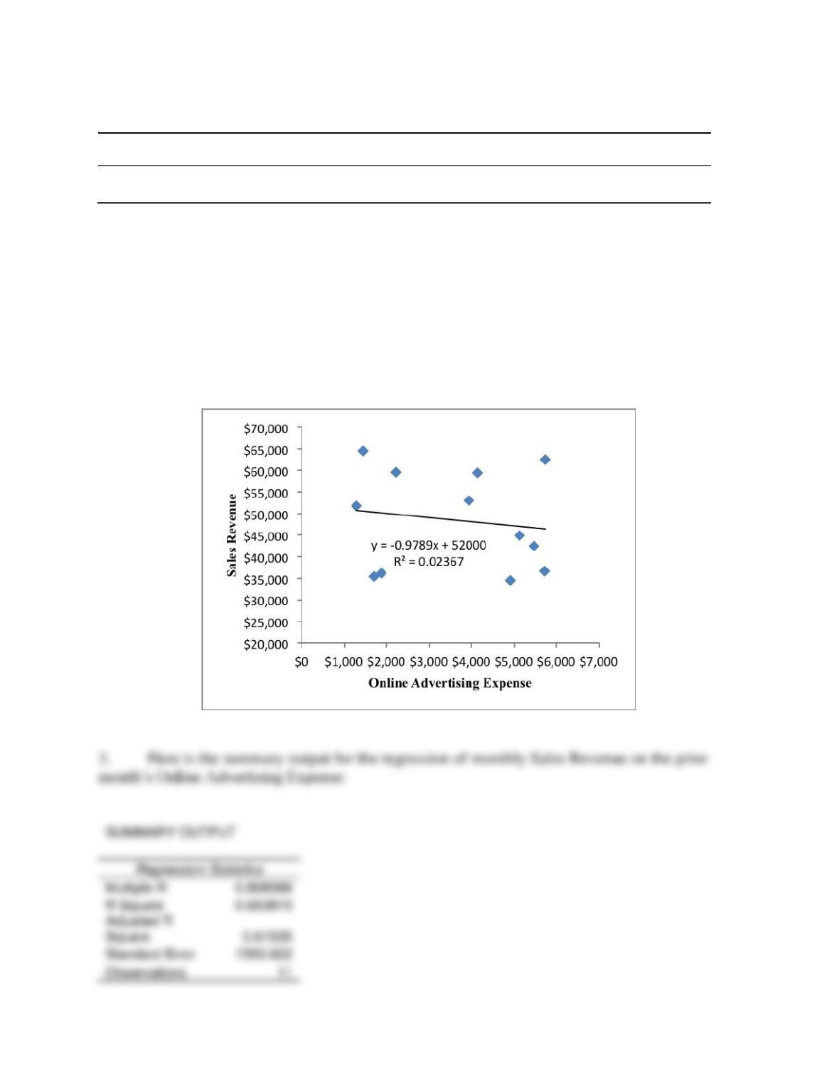
2. SOLUTION EXHIBIT 10-41A presents the data plot for the initial analysis. The formula
of Sales Revenue = $52,000 – (0.98 × Online advertising expense) indicates that there is a fixed
amount of revenue each month of $52,000, which is reduced by 0.98 times that month’s online
advertising expense. This relationship is not economically plausible, as advertising would not
reduce revenue. The data points do not appear linear, and the r-square of 0.02 indicates a very
weak goodness of fit (in fact, almost no fit at all).
SOLUTION EXHIBIT 10-41 A
Plot and Regression Line for Sales Revenue and Online Advertising Expense
SUMMARY OUTPUT
Multiple R
0.808588
R Square
0.653815
10-71
ANOVA
df
SS
MS
F
Significance
F
Regression
1
9.29E+08
929262059
16.99763
0.002587
Residual
9
4.92E+08
54670085
Total
10
1.42E+09
Coefficients
Standard
Error
t Stat
P-value
Lower 95%
Upper
95%
Intercept
28361.37
5428.687
5.2243522
0.000546
16080.83
40641.91
X Variable 1
5.381665
1.305336
4.1228186
0.002587
2.428789
8.33454
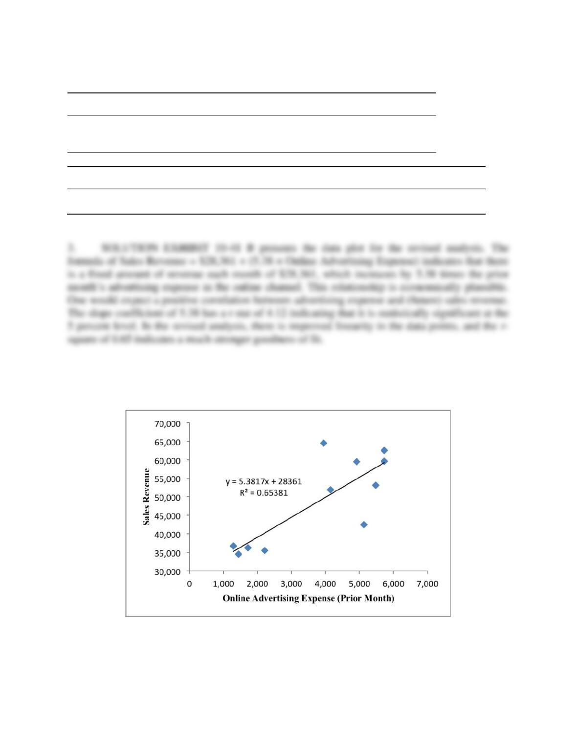
SOLUTION EXHIBIT 10-41B
Plot and Regression Line for Sales Revenue and Previous Month Online Advertising
4. Nandita must be very careful about making conclusions regarding cause and effect. Even
a strong goodness of fit does not prove a cause and effect relationship. The independent and