CHAPTER 10/HYPOTHESIS TESTING: CATEGORICAL DATA 237
Missing 1 2 3
All 171 273 444
Tabulated statistics: Mat_curr, elbow
Rows: Mat_curr Columns: elbow
0 1 All
Wood 50 62 112
Tabulated statistics: Str_curr, elbow
Rows: Str_curr Columns: elbow
0 1 All
To test for an effect of gender, we construct a 2×2 table and use the Chi-Square test statistic
. tabulate sex elbow, chi2
| elbow
Sex | 0 1 | Total
———–+———————-+———-
For the “type” and “weight” variables, we note that a natural ordering exists, and so we decide to use Chi-
Square trend tests, excluding observations listed as either “missing” or “don’t know” . (“Don’t know” was
only reported 4 times in the data set).
. nptrend elbow if typ_curr<4, by( typ_curr )
typ_curr score obs sum of ranks
238 CHAPTER 10/HYPOTHESIS TESTING: CATEGORICAL DAT
A
For the variables relating to racquet material and string type, we elect to use the Chi-Square test for
. tabulate mat_curr elbow if mat_curr<9, chi2 row
| elbow
Mat_curr | 0 1 | Total
———–+———————-+———-
Wood | 50 62 | 112
| 44.64 55.36 | 100.00
———–+———————-+———-
. tabulate mat_curr elbow if mat_curr<6, chi2 row
| elbow
Mat_curr | 0 1 | Total
———–+———————-+———-
Wood | 50 62 | 112
| 44.64 55.36 | 100.00
. tabulate str_curr elbow if str_curr<3, chi2 row
| elbow
Str_curr | 0 1 | Total
CHAPTER 10/HYPOTHESIS TESTING: CATEGORICAL DATA 239
10.60 For this question, we use only observations 1-128. Using MINITAB to perform and 2-sample test for
binomial proportions, we find a significantly greater clearance rate associated with CEF (Antibo=1).
Test and CI for Two Proportions: Clear_1, Antibo_1
Event = 1
Antibo_1 X N Sample p
Cef 38 62 0.612903
10.61 Having created a new variable “clear2” measuring our ordered response, we can create a 2×3 table.
Using either the Chi-Square test for trend or for heterogeneity, we find no significant association between
outcomes and antibiotic assignment. We note that the trend test is preferred, and that the heterogeneity test
is shown only as additional information.
nptrend antibio in 1/75, by( clear2 )
clear2 score obs sum of ranks
0 0 29 1215
| Antibio
Clear2 | 1 2 | Total
———–+———————-+———-
0 | 14 15 | 29
240 CHAPTER 10/HYPOTHESIS TESTING: CATEGORICAL DAT
A
10.62 Out of 75 children with two affected ears (or 150 total ears), we find 1×12 + 2×34 = 12+68 = 80 total
cleared ears, for a total clearance rate of 80/150 = 53.3%. Under the assumption of independence, the
10.63 This is a matched pair study involving binomial proportions. Thus, McNemar’s test for correlated
10.64 We wish to test the hypothesis : vs. : , where (discordant pair is of
type A). In this context a type A discordant pair is a pair where the case reports an adverse event and the
have adverse events than controls.
10.65 We can organize the data into a 2 u 5 table. We can approximate the counts in the table as follows:
H0p 12 H1pz12 p prob
O
O
11
16 353 34 5560
16 353 23 3761
,.
,.
CHAPTER 10/HYPOTHESIS TESTING: CATEGORICAL DATA 241
Since , we subtract 1 from the largest count to
obtain the correct total (77,220). The observed table is as follows:
parity
0 1 2 3 4+
induced yes 5,560 3,761 4,906 1,635 491 16,353
10.66 We have the test statistic , where
A 5560 0
3761 1
4906 2
1635 3
491 4
Thus,
10.67 Suppose the incidence of breast cancer is x among nulliparous women. It follows from the conditions of
the problem that the incidence of breast cancer for women with 1 child , 2 children ,
OOOOO
21 22 23 24 25 77,221 26 255 1 26 254,,
XAB
1
22
.9
x
..981
2xx
242 CHAPTER 10/HYPOTHESIS TESTING: CATEGORICAL DAT
A
10.69 The test statistic for this test is
10.70 We wish to compute the test statistic
Thus, we have the following table:
igroup
OiEi
CHAPTER 10/HYPOTHESIS TESTING: CATEGORICAL DATA 243
10.71 The proportion of people who developed abnormal triglyceride levels was
10.72 We have the following 2 u 2 table:
abnormal triglyceride levels
group yes no
10.73 We calculate the expected count in each cell as follows:
The test statistic is
244 CHAPTER 10/HYPOTHESIS TESTING: CATEGORICAL DAT
A
10.74 We form a 2 u 2 table relating the type of bird to the type of sunflower seeds eaten:
Type of seed
Type of Bird black oil striped total
Titmouse 1 4 5
10.75 To perform this test, we first enumerate all possible tables with the same row and column margins as the
observed table:
10.76 We display the observed and expected counts in a 2 u 4 table as shown below (expected counts in
Day
1 2 3 4 Total
10.77 The expected value for the
E
cell (listed in parentheses in the above table) is obtained from
05
14
23
32
41
50
CHAPTER 10/HYPOTHESIS TESTING: CATEGORICAL DATA 245
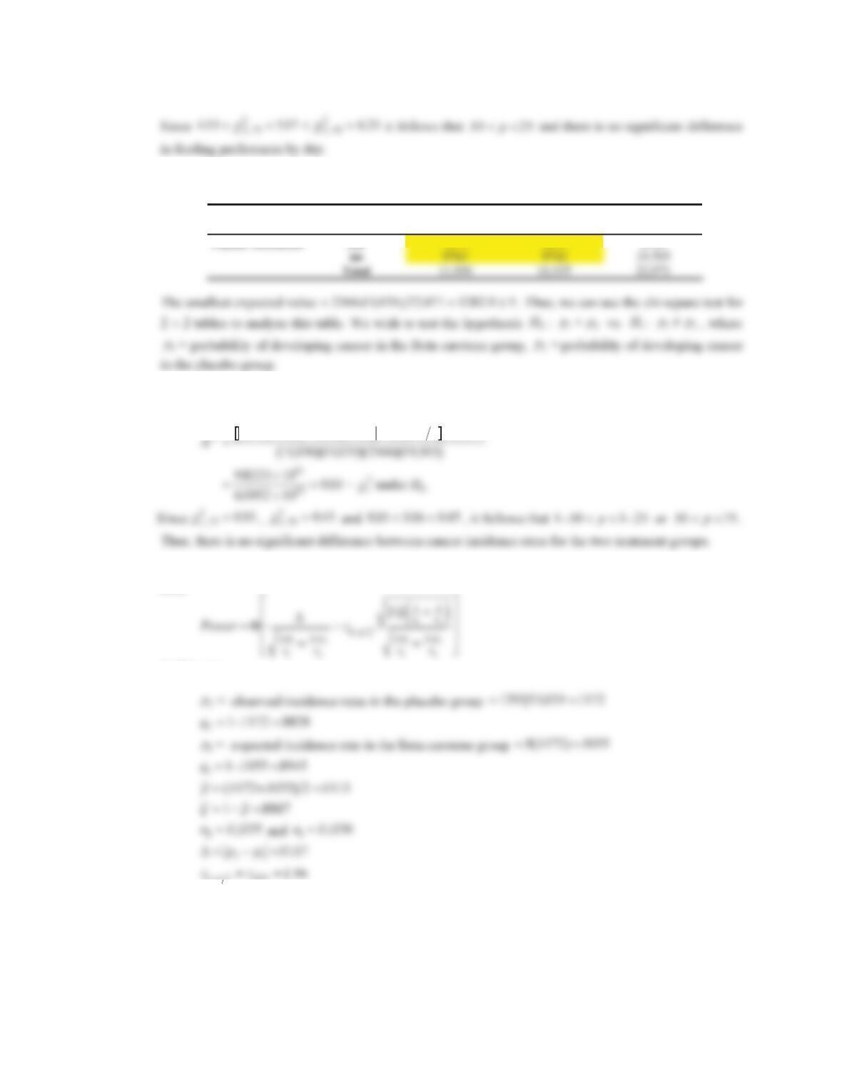
10.78 We have the following 2 u 2 table relating cancer incidence to treatment group:
Treatment Group
Beta carotene Placebo total
Cancer Incidence yes 1273 1293 2566
10.79 We have the test statistic
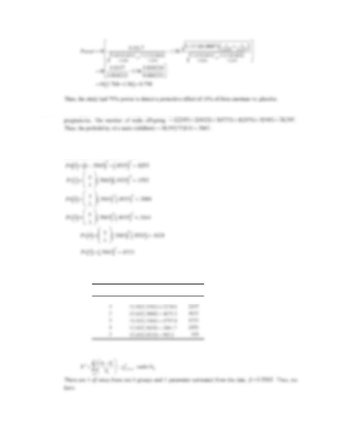
10.80 We use the power formula for comparing two binomial proportions (see Equation 10.15 in Chapter 10,
text)
In this case,
12 .975
D
Therefore, the power is given by:
2
2
1273 9742 1293 9763 22,071 2 22,071
246 CHAPTER 10/HYPOTHESIS TESTING: CATEGORICAL DAT
A
10.81 If the gender of successive offspring are independent, then we have independent
10.82 If the gender of successive pregnancies within a family are independent, then the number of male
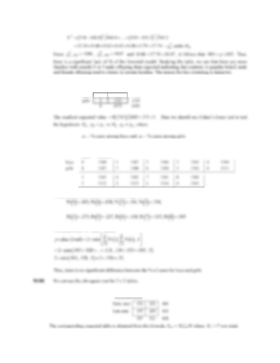
offspring is binomial with parameters, and . To compute the probability of 0, 1, }, 5
male births, we use Excel. We have:
10.83 If the gender of successive offspring are independent, then the expected number of families of size 5
(15,162) with 0, 1, }, 5 male offspring is given in the E column of the following table
Number of Male
Offspring E O
0
15,162 .0293 444.0 518
We now perform the chi-square goodness-of-fit test using the test statistic
15162 5 75 810,,u
n 5p .5065
CHAPTER 10/HYPOTHESIS TESTING: CATEGORICAL DATA 247
10.84 We have the following 22utable
cases controls
10.85 We have to enumerate all tables with the same margins as the observed table as follows
cases controls
The probabilities of each of these tables is given by
We observe the “6” table. Hence,
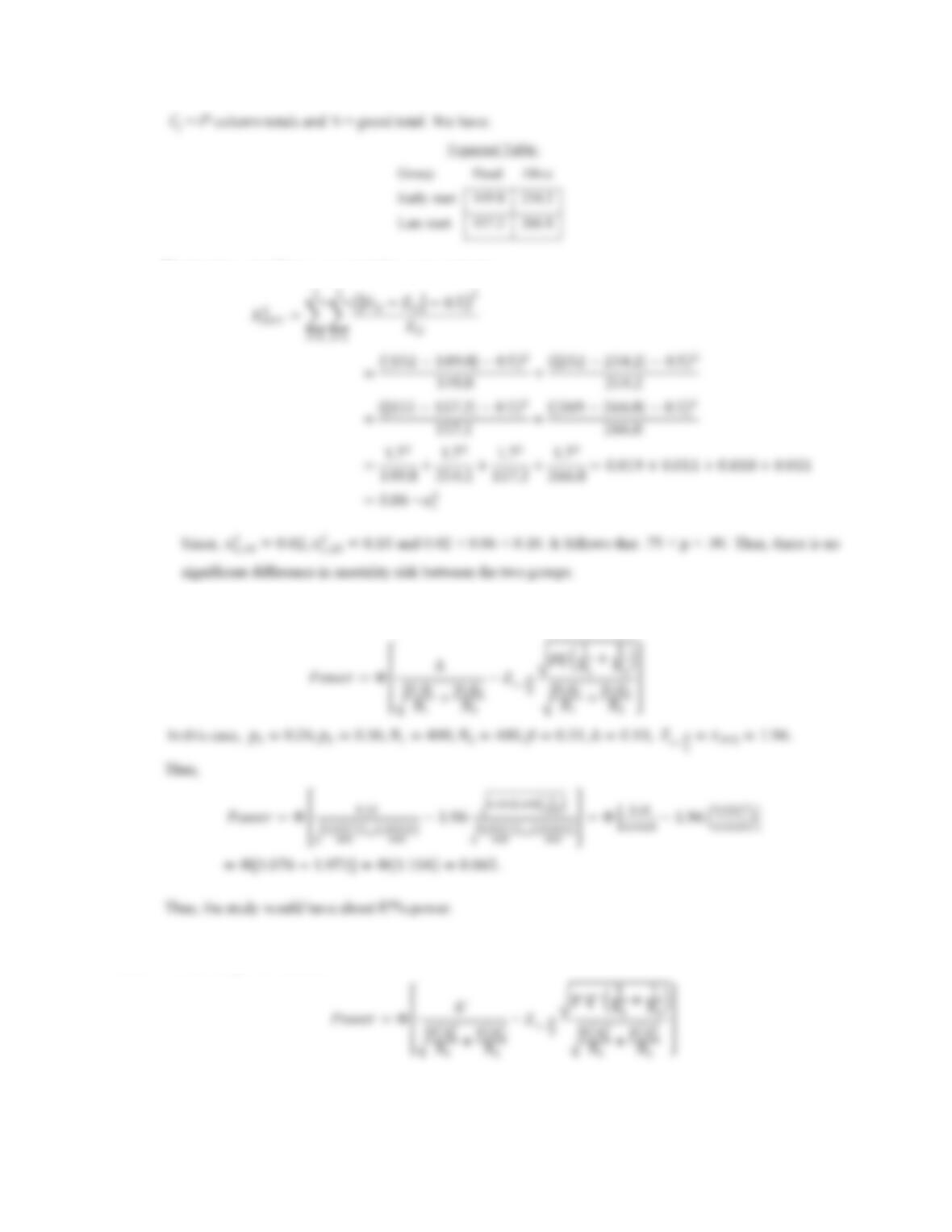
10.87 We have the following observed 2 x 2 table:
Observed Table:
248 CHAPTER 10/HYPOTHESIS TESTING: CATEGORICAL DAT
A
We then have the Yates-corrected chi-square statistic:
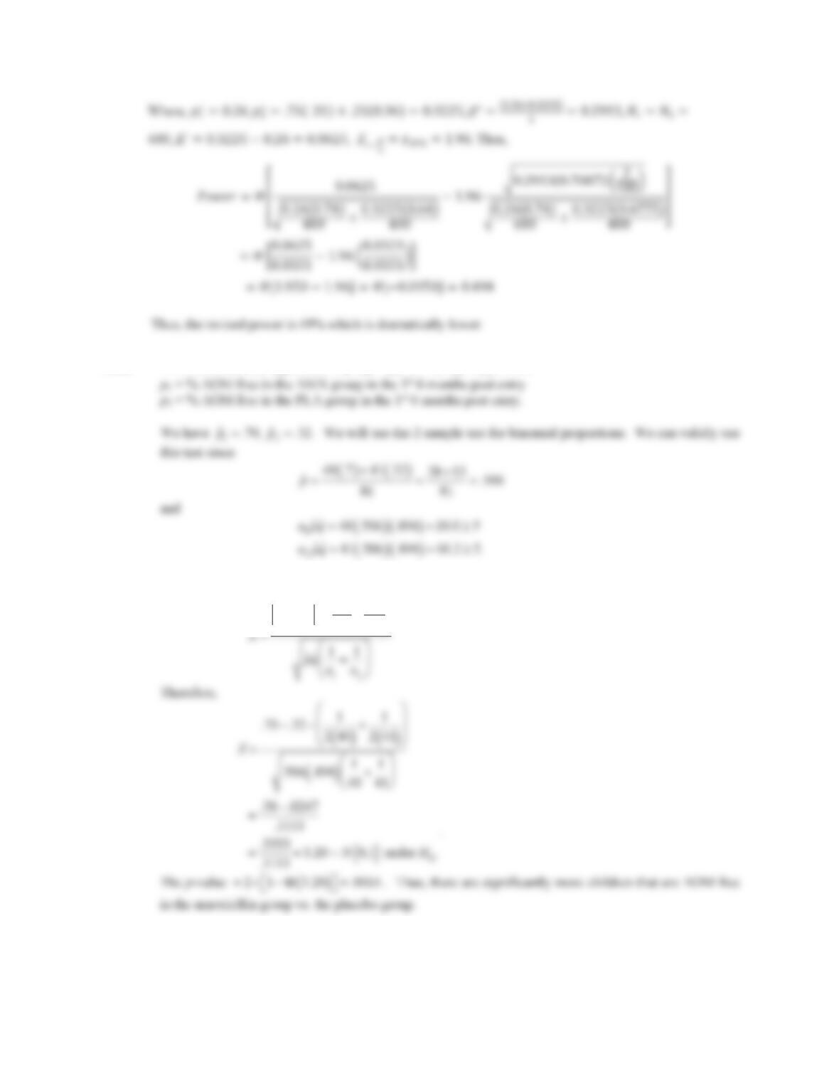
10.88 We use the power formula:
10.89 We use the power formula:
CHAPTER 10/HYPOTHESIS TESTING: CATEGORICAL DATA 249
10.90 We wish to test the hypothesis 01 2 11 2
:vs.:
H
pp Hpp z, where
10.91 The test statistic is
ˆ
p
1
ˆ
p
2
1
2n1
1
2n2
§
©
¨
¨
·
¹
¸
¸
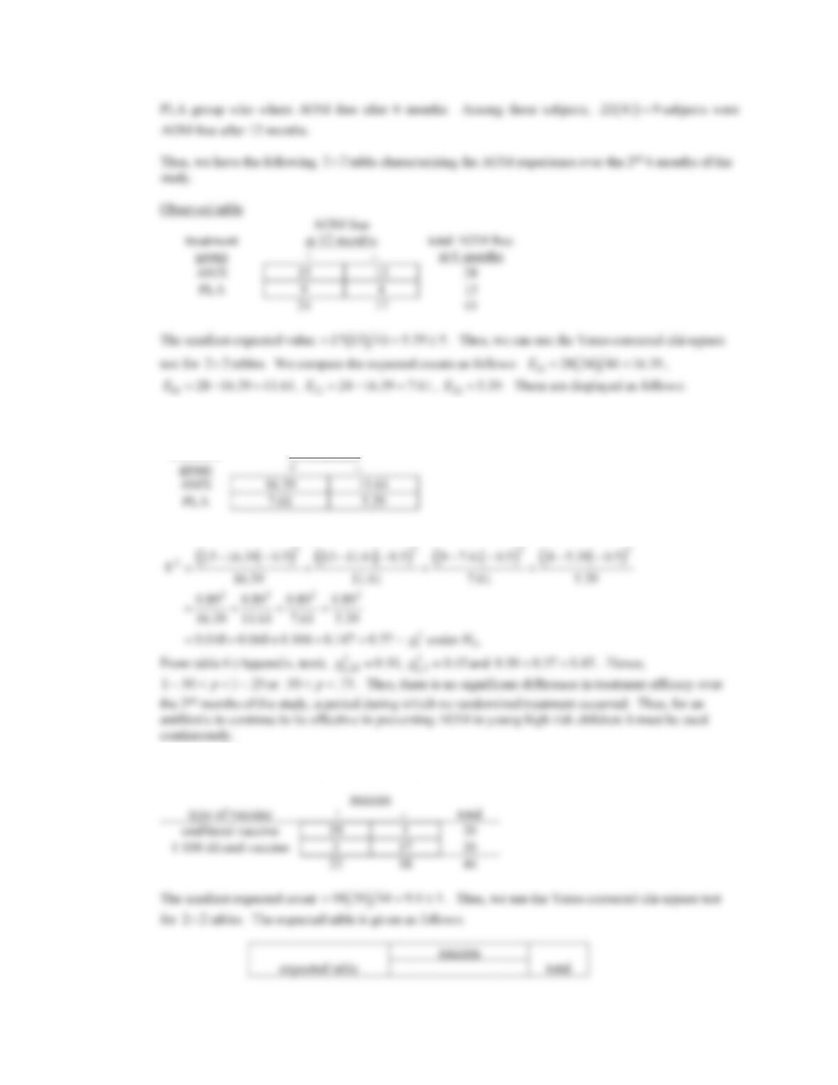
10.92 There were
.7 40 28 subjects in the AMX group who where AOM free after 6 months. Among these
subjects,
.38 40 15 subjects were AOM free after 12 months. There were
.32 41 13 subjects in the
250 CHAPTER 10/HYPOTHESIS TESTING: CATEGORICAL DAT
A
Expected table
treatment
AOM free
at 12 months
We have the test statistic
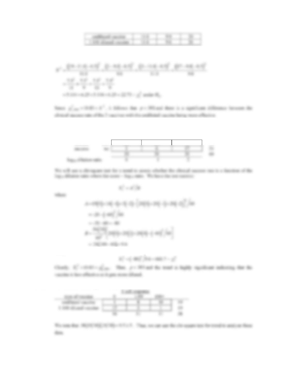
10.93 We form a 22utable relating success rate to type of vaccine as follows:
CHAPTER 10/HYPOTHESIS TESTING: CATEGORICAL DATA 251
Thus the chi-square statistic is given by
10.94 We have the following 23utable
type of vaccine
undiluted 1:10 diluted 1:100 diluted total
clinical yes 19 14 3 36
Thus,
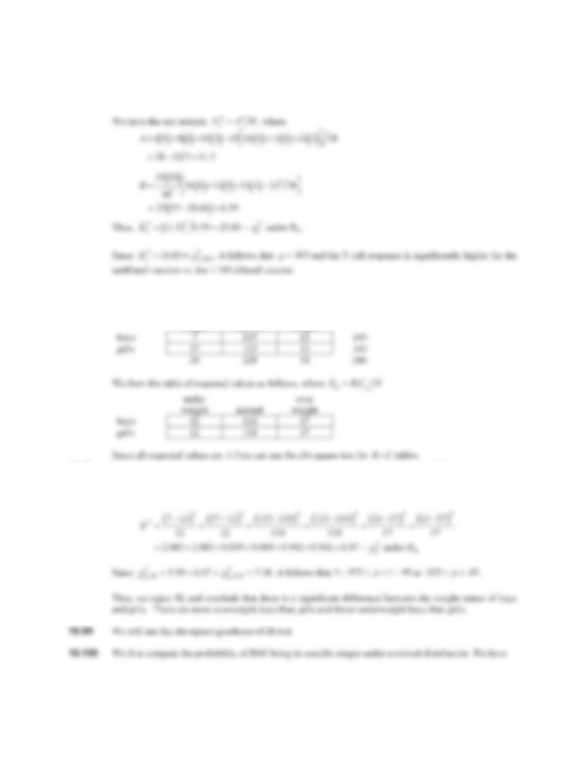
10.95 We have the following 23utable
252 CHAPTER 10/HYPOTHESIS TESTING: CATEGORICAL DAT
A
10.96 For simplicity, we will use scores of 0, 1, 2 for the T cell response groups 0, 1-99, and 100+,
respectively.
10.97 We have the following 23utable
under
weight normal
over
weight
10.98 We wish to test the hypothesis 01
:vs.:
ij ij ij ij
H
pab Hpab z
where pij = probability of being in the
ith row and jth column, ai = probability of being in the ith row and bj = probability of being in the jth
column. We have: