Chapter 10 Budgetary Planning and Control
10–17
Super Clean Inc.
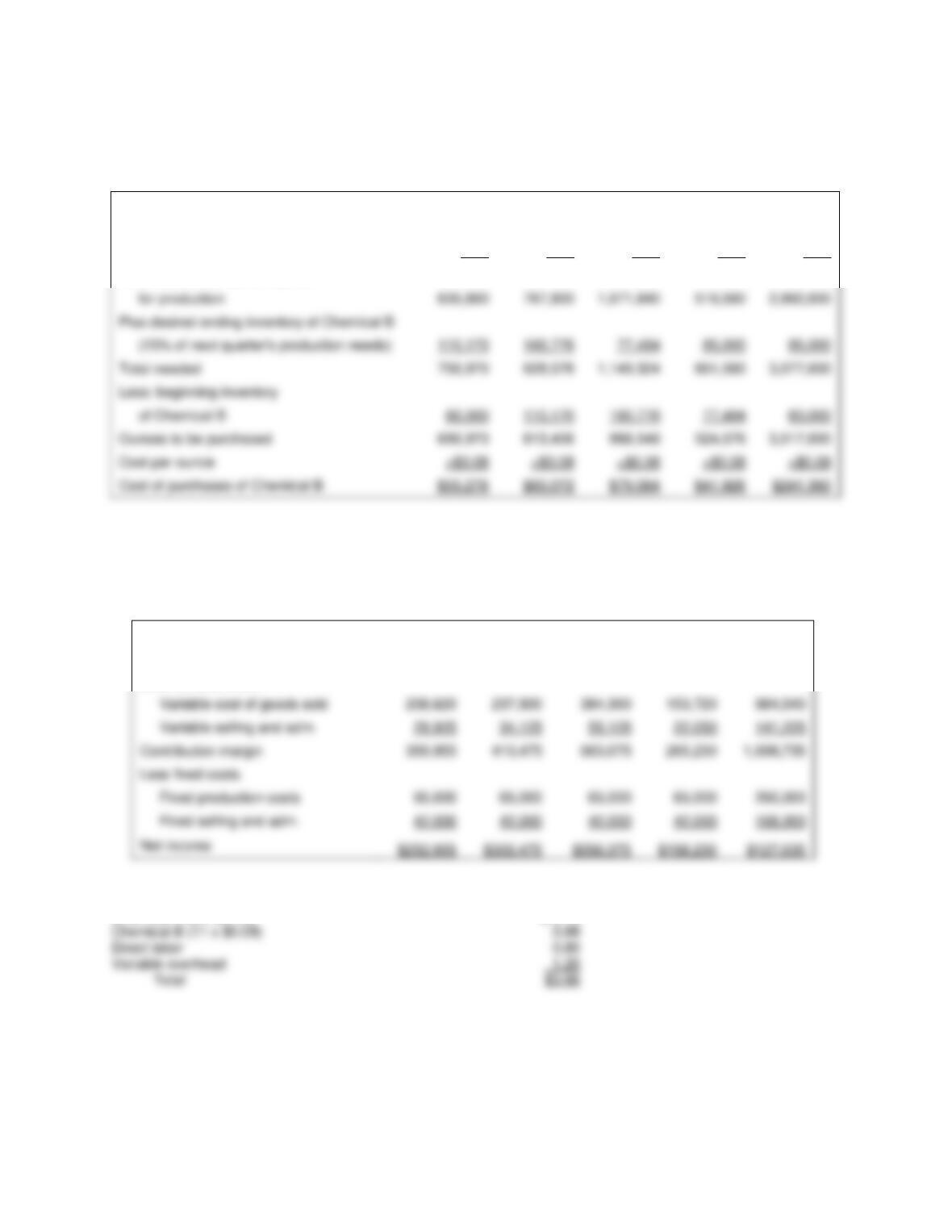
Material Purchases Budget for 2018
Chemical B
Quarter 1
Quarter 2
Quarter 3
Quarter 4
Year
Units to be produced
57,800
69,800
97,440
46,960
272,000
Ounces of Chemical B per unit
× 11
× 11
× 11
× 11
× 11
Ounces of Chemical B required
c.
Super Clean Inc.
Budgeted Income Statement for the Year 2018
Quarter 1
Quarter 2
Quarter 3
Quarter 4
Year
Sales
$598,500
$682,500
$1,102,500
$441,000
$2,824,500
Less variable costs:
Contribution margin
Less fixed costs
Variable cost of sales per bottle:
Chemical A (6 x $0.13) $ 0.78
635,800
767,800
516,560
Plus desired ending inventory of Chemical B
115,170
160,776
77,484
85,000
85,000
Total needed
750,970
928,576
601,560
Less: beginning inventory
60,000
115,170
160,776
77,484
60,000
Ounces to be purchased
690,970
813,406
988,548
524,076
Cost per ounce
×$0.08
×$0.08
×$0.08
×$0.08
×$0.08
Cost of purchases of Chemical B
P9. [LO 2]
a.
Fenzel Slide Oil
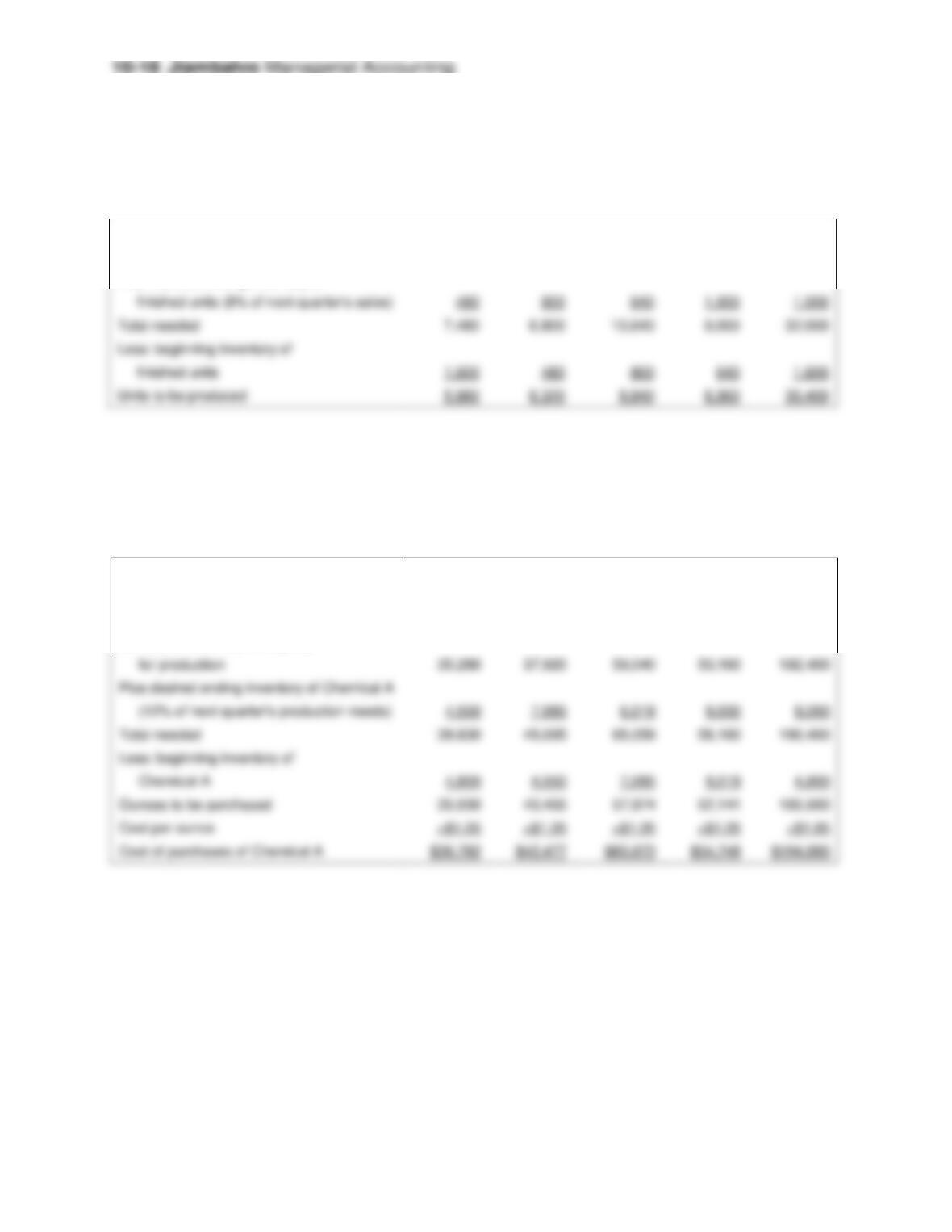
Production Budget for 2018
Quarter 1
Quarter 2
Quarter 3
Quarter 4
Year
Unit sales
7,000
6,000
10,000
8,000
31,000
Plus: Desired ending inventory of
Total needed
Less: beginning inventory of
Units to be produced
b.
Fenzel Slide Oil
Material Purchases Budget 2018
Chemical A
Quarter 1
Quarter 2
Quarter 3
Quarter 4
Year
Units to be produced
5,880
6,320
9,840
8,360
30,400
Ounces of Chemical A per unit
6
6
6
6
6
Ounces of Chemical A required
59,040
Plus desired ending inventory of Chemical A
4,550
7,085
6,019
8,000
8,000
Total needed
65,059
Less: beginning inventory of
4,800
4,550
7,085
6,019
4,800
Ounces to be purchased
57,974
Cost per ounce
×$1.05
×$1.05
Cost of purchases of Chemical A
Chapter 10 Budgetary Planning and Control
10–19
Fenzel Slide Oil
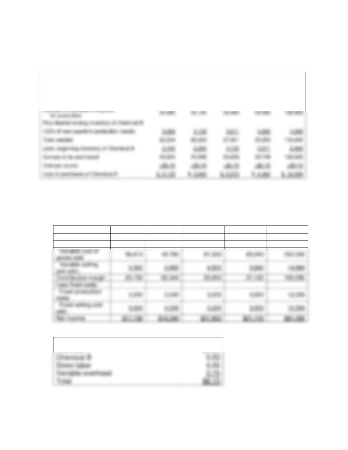
Material Purchases Budget 2018
Chemical B
Quarter 1
Quarter 2
Quarter 3
Quarter 4
Year
Units to be produced
5,880
6,320
9,840
8,360
30,400
Ounces of Chemical B per unit
3.5
3.5
3.5
3.5
3.5
c.
Fenzel Slide Oil
Budgeted Income Statement for the Year 2018
Quarter 1
Quarter 2
Quarter 3
Quarter 4
Year
Sales
$84,000
$72,000
$120,000
$96,000
$372,000
Less variable costs:
Contribution margin
20,340
Less fixed costs:
costs
Net income
$17,730
$14,340
$27,900
$21,120
Variable cost of sales per bottle:
Chemical A
$6.30
Chemical B
Direct labor
Variable overhead
Total
$8.13
Jiambalvo Managerial Accounting
10–20
P10. [LO 2]
Casey Wholesalers
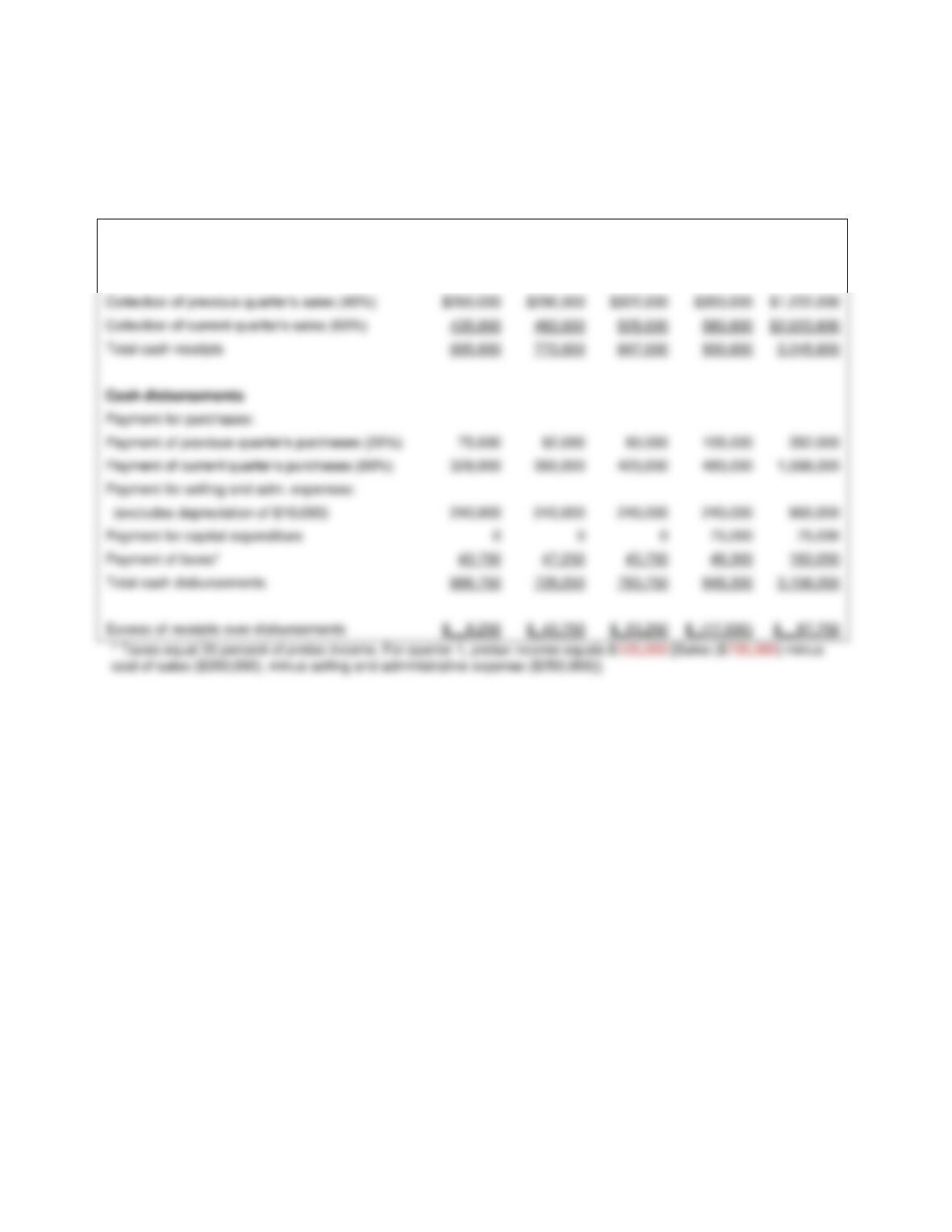
Cash Budget for the Year 2018
Quarter 1
Quarter 2
Quarter 3
Quarter 4
Year
Cash receipts
Collection of credit sales:
$1,222,000
$2,023,800
Total cash receipts
Cash disbursements
Payment for purchases:
Payment of previous quarter’s purchases (20%)
Payment for selling and adm. expenses:
Payment for capital expenditure
0
Payment of taxes*
Total cash disbursements
Excess of receipts over disbursements
$_(17,500)
P11. [LO 2]
Eurofit Cycling
Cash Budget for the Year 2018
Total cash receipts
Cash disbursements
Payment for purchases:
Payment of previous quarter’s purchases (30%)
Payment of current quarter’s purchases (70%)
Payment for capital expenditure
Payment of taxes*
Total cash disbursements
Excess of receipts over disbursements
Quarter 1
Quarter 2
Quarter 3
Quarter 4
Year
Cash receipts
Collection of credit sales:
Collection of previous quarter’s sales (50%)
$275,000
$200,000
$237,500
$275,000
$ 987,500
P12. [LO 2]
Step 1 Expected sales in 2018 = (1.25 x sales of the same quarter previous year)
Step 2 Cost of sales = (.75 x Expected Sales)
Q1, 2018
Q2, 2018
Q3, 2018
Q4, 2018
Year
Q1, 2019
Sales in 2017
Expected sales in 2018
$1,517,500
$300,000
Plus Ending inventory
Less Beginning inventory
_120,750
$250,000
$300,000
$290,000
$368,000
$1,208,000
P13. [LO 2]
Results for basic assumption:
Q1, 2017 Q2, 2017 Q3, 2017 Q4, 2017
Sales growth 8%
Q1, 2018
Q2, 2018
Q3, 2018
Q4, 2018
Q1, 2019
Sales
$274,320
$297,000
$345,600
$221,400
$296,666
Cost of sales
Less beginning inventory
Purchases
_$83,805
_$81,420
Chapter 10 Budgetary Planning and Control
10–23
Results for combination 1:
Q1, 2017 Q2, 2017 Q3, 2017 Q4, 2017
Sales $254,000 $275,000 $320,000 $205,000
Sales growth 10%
Desired ending inventory % 22%
Cost of sales % 33%
Q1, 2018
Q2, 2018
Q3, 2018
Q4, 2018
Q1, 2019
Sales
$279,400
$302,500
$352,000
$225,500
$307,340
Results for combination 2:
Q1, 2017 Q2, 2017 Q3, 2017 Q4, 2017
Sales $254,000 $275,000 $320,000 $205,000
Q1, 2018
Q2, 2018
Q3, 2018
Q4, 2018
Q1, 2019
Sales
Cost of sales
Plus desired ending inventory
Less beginning inventory
Purchases
Plus desired ending inventory
Less beginning inventory
Purchases
$103,419
$106,976
Jiambalvo Managerial Accounting
10–24
Results for combination 3:
Q1, 2017 Q2, 2017 Q3, 2017 Q4, 2017
Sales $254,000 $275,000 $320,000 $205,000
Sales growth 9%
Q1, 2018
Q2, 2018
Q3, 2018
Q4, 2018
Q1, 2019
Sales
$276,860
$299,750
$348,800
$223,450
$301,777
Plus desired ending inventory
Less beginning inventory
Purchases
$123,710
$126,571
$122,472
$100,033
P14. [LO 3]
a. Both individuals are fighting for their self-interests, which are in conflict. Debra
wants budgeted revenue low and budgeted expenses high so that she can
b. One option for the President is to ask Debra and Barney to bring all relevant
P15. [LO 1, 2, 3]
a. Assumptions:
Salaries of customer consultants are variable costs. Salaries of supervisors,
office space expense, and depreciation are fixed costs.
14,000 calls
14,000 calls
Flex. Budget
Actual
Variance
Salaries of customer consultants
$200,000
$182,000
$18,000
Salaries of supervisors
Office space charge
Depreciation of equipment
Chapter 10 Budgetary Planning and Control
10–25
b. It appears that variances for salaries of customer consultants and depreciation
of equipment are significant variances at about 9 percent and 14 percent of the
flexible budget amounts.
Some possible explanations:
c. Relevant non-financial measures might include: number of calls answered,
P16. [LO 3]
The variances are “favorable” because the budget has not been adjusted for the
P17. [LO 3]
a. Budget padding involves biasing estimates of sales downward and expenses
upward so that actual profit is more likely to exceed budgeted profit. Franz has
b. The budget was set at $45,000,000 and budget compensation is capped when
P18. [LO 1]
Listed below are four possible measures. There are other possibilities as well.
1. Customer satisfaction rating based on market survey data

Jiambalvo Managerial Accounting
10–26
Case 10-1 [LO 3, Ethics]
COLUMBUS PARK – WASTE TREATMENT FACILITY
Summary
A manager of a water treatment facility is submitting a budget for an amount higher
than the expected cost because she expects the budget to be cut by the city controller.
• Focuses on ethical considerations related to budgeting
Questions to ask students
1. What is the situation facing Ann Paxton at the Columbus Park Waste Treatment
Facility?
2. Is it ethical to submit a padded budget because you expect it to be cut?
Discussion
Ann Paxton is the manager of the Columbus Park Waste Treatment Facility. She
expects costs to be $4,200,000 but is going to submit a budget of $4,900,000 because
she expects the city controller to cut her budget by 10 percent.

Case 10-2 [LO 2]
ABRUZZI OLIVE OIL COMPANY
Summary
A small producer of olive oil is preparing budgets to consider the impact of various
sales levels.
• Relatively straightforward spreadsheet case.
• Refocuses student attention on the contribution margin.
Questions to ask students:
1. What is the situation facing Abruzzi Olive Oil Company?
2. Present the six monthly budget schedules Cheryl suggested (budgets with and
without Consolidated business on top of increases of 5%, 10%, and 15%).
3. What is the impact on profit of obtaining the Consolidated business (assuming
there is not a capacity constraint)?
Discussion
What is the decision facing Abruzzi Olive Oil Company? The owner, Cheryl Sounders,
Jiambalvo Managerial Accounting
10–28
a. Present the six monthly budget schedules Cheryl suggested (budgets with and
without Consolidated business on top of increases of 5%, 10%, and 15%).
The first step is to build sales budgets with and without the Consolidated business.
2018
2018
2018
2017
5%
increase
10%
increase
15%
increase
January
9,200
9,660
10,120
10,580
February
9,000
9,450
9,900
10,350
March
9,400
9,870
10,340
10,810
Add 1,250 to each month for Consolidated business
January
10,910
11,370
11,830
February
10,700
11,150
11,600
March
April
10,280
10,710
11,140
May
9,650
10,050
10,450
June
10,175
10,600
11,025
July
9,860
10,270
10,680
August
9,125
9,500
9,875
September
10,595
11,040
11,485
October
11,015
11,480
11,945
November
10,910
11,370
11,830
December
11,330
11,810
12,290
11,120
11,590
12,060
April
8,600
9,030
9,460
9,890
May
8,000
8,400
8,800
9,200
June
8,500
8,925
9,350
9,775
July
8,200
8,610
9,020
9,430
August
7,500
7,875
8,250
8,625
September
8,900
9,345
9,790
10,235
October
9,300
9,765
10,230
10,695
November
9,200
9,660
10,120
10,580
December
9,600
10,080
10,560
11,040
Chapter 10 Budgetary Planning and Control
10–29
The second step is to build production budgets based on the sales budgets. First, we
do this without the extra sales to Consolidated. Note the calculation of ending
inventory in December with 5% growth in sales is 12 % of December sales (.12 x
10,080 = 1,210).
5%
Sales
EI
BI
Production
January
9,660
1,134
1,500
9,294
February
9,450
1,184
1,134
9,500
10%
Sales
EI
BI
Production
January
10,120
1,188
1,500
9,808
February
9,900
1,241
1,188
9,953
March
10,340
1,135
1,241
April
9,460
1,056
1,135
9,381
May
8,800
1,122
1,056
8,866
June
9,350
1,082
1,122
9,310
July
9,020
1,082
8,928
August
8,250
1,175
8,435
September
9,790
1,228
1,175
9,843
October
10,230
1,214
1,228
November
10,120
1,267
1,214
December
10,560
1,267
1,267
March
9,870
1,084
1,184
9,769
April
9,030
1,008
8,954
May
8,400
1,071
1,008
8,463
June
8,925
1,033
1,071
8,887
July
8,610
1,033
8,522
August
7,875
1,121
8,051
September
9,345
1,172
1,121
9,395
October
9,765
1,159
1,172
9,752
November
9,660
1,210
1,159
9,710
December
10,080
1,210
1,210

Jiambalvo Managerial Accounting
10–30
15%
Sales
EI
BI
Production
January
10,580
1,242
1,500
10,322
February
10,350
1,297
1,242
10,405
March
10,810
1,187
1,297
10,700
April
1,104
1,187
May
1,173
1,104
June
1,132
1,173
July
1,035
1,132
August
1,228
1,035
September
10,235
1,283
1,228
10,290
October
10,695
1,270
1,283
10,681
November
10,580
1,325
1,270
10,635
December
11,040
1,325
1,325
11,040
Then, we redo the analysis, with the extra sales to Consolidated.
5%
Sales
EI
BI
Production
January
10,910
1,284
1,500
10,694
February
10,700
1,334
1,284
10,750
March
11,120
1,234
1,334
11,019
April
10,280
1,158
1,234
10,204
May
1,221
1,158
June
10,175
1,183
1,221
10,137
July
1,095
1,183
August
1,271
1,095
September
10,595
1,322
1,271
10,645
October
11,015
1,309
1,322
11,002
November
10,910
1,360
1,309
10,960
December
11,330
1,360
1,360
11,330
10%
Sales
EI
BI
Production
January
11,370
1,338
1,500
11,208
February
11,150
1,391
1,338
11,203
March
11,590
1,285
1,391
11,484
April
10,710
1,206
1,285
10,631
May
June
10,600
1,232
1,272
10,560
July
10,270
1,140
1,232
10,178
August
1,325
1,140
September
11,040
1,378
1,325
11,093
October
11,480
1,364
1,378
11,467
November
11,370
1,417
1,364
11,423
11,810
1,417
1,417
11,810
10,050
1,272
1,206
10,116
15%
Sales
EI
BI
Production
January
11,830
1,392
1,500
11,722
February
11,600
1,447
1,392
11,655
March
12,060
1,337
1,447
11,950
April
11,140
1,254
1,337
11,057
May
10,450
1,323
1,254
10,519
June
11,025
1,282
1,323
10,984
July
10,680
1,185
1,282
10,583
August
1,378
1,185
10,068
September
11,485
1,433
1,378
11,540
October
11,945
1,420
1,433
11,931
11,830
1,475
1,420
11,885
December
12,290
1,475
1,475
12,290
Jiambalvo Managerial Accounting
10–32
c. What is the impact on profit of obtaining the consolidated business (assuming there
is not a capacity constraint)? Consolidated will purchase 15,000 gallons per year.