CHAPTER 10: Standard Costing and Variance Analysis
P 10-68 (Concluded)
8.0
LRV:
8.0
LEV:
CHAPTER 10 Standard Costing and Variance Analysis
P 10-69
change here, please →
1. MPV = (AP – SP)AQ ↓ links ↓ links ↓ Std. qty. Std.Price Std.cost
= ($1.55 – $1.50)44,250 = $2,213* U 1.55
–
1.50
×
44,250
=
2,213 U DM 0.50 1.50 0.75 2,213
* Rounded to the nearest dollar.
MUV = (AQ – SQ*)SP DL 0.15 10 1.50 U
= (44,250 – 45,000)$1.50 = $1,125 F 44,250
–
45,000
×
1.50
=
(1,125) F No. of weeks in a year 52 (1,125)
The overall materials variance is $1,088 U ($2,213 U – $1,125 F); therefore, the 2,213
–
(1,125)
=
1,088 U Units produced 90,000 F
company should not buy this quality of materials, but should go back to Actual labor costs 138,000
the prior quality. Actual labor hours 13,400
×
=
–
×
=
×
–
×
=
The overall labor variance is $3,000 U ($4,000 U – $1,000 F). If this pattern is 4,000
–
=
expected to persist, then the new layout should be abandoned.
3. LRV = (AR × AH) – (SR × AH)
= Actual Labor Cost – (SR × AH) ↓ links ↓ links ↓
= $132,000 – ($10 × 13,200) = $0 132,000
–
10
×
13,200
=
0
LEV = (SR × AH) – (SR × SH**)
= ($10 × 13,200) – ($10 × 13,500) = $3,000 F 10
×
13,200
–
10
×
13,500
=
(3,000) F (3,000) F
** SH = 90,000 × 0.15 = 13,500 *90,000
×
0.15
=
(13,500)
The overall labor variance is $3,000 F ($0 + $3,000 F). If this pattern is the one 0
+
(3,000)
=
(3,000) F
expected to persist, then the new layout should be continued. It will save
$156,000 per year ($3,000 × 52 weeks). (3,000)
×
52
=
(156,000)
P 10-70
change here, please →
1. MPV = (AQ × AP) – (SP × AQ) Direct materials 4
= Actual Materials Cost – (SP × AQ) ↓ links ↓ links ↓ Direct labor 23
= $74,000 – ($0.95)78,000 = $100 F 74,000
–
0.95
×
78,000
=
(100) F Std. qty. of lbs. reqd. 4 (100)
MUV = (AQ – SQ*)SP Std. price per lbs. 0.95 F
= (78,000 – 60,000)($0.95) = $17,100 U 78,000
–
60,000
×
0.95
=
17,100 U Std. hrs. reqd. 1.25 17,100
Overall Materials Variance = $100 F + $17,100 U = $17,000 U (100)
+
17,100
=
17,000 U Std. wage rate 15.00 U
×
=
–
×
=
×
–
×
=
×
=
CHAPTER 10: Standard Costing and Variance Analysis
P 10-70 (Concluded)
3. The basic advantages offered by a standard costing system include its
use in planning, control, and decision making. A standard costing system
helps in budgeting since the unit standard costs can be multiplied by the
predicted level of production to obtain total costs. Standard costs are
used in control to evaluate performance. A comparison of actual costs to
standard costs allows management to evaluate the performances of cost
centers. Finally, standard costs assist in decision making. For example,
having standard costs can make pricing decisions easier.
Standard costing systems also have disadvantages. For example,
standards that are set too high (e.g., theoretical or perfect standards) can
cause motivation to decrease, as workers believe that they can never
achieve the standards. Standards may also stand in the way of continual
improvement if they are not updated frequently to adjust for gradual
increases in efficiency.
P 10-71
change here, please →
1. MPV = (AP – SP)AQ ↓ links ↓ links ↓ Direct materials 30.00
= ($4.70 – $5.00)260,000 = $78,000 F 4.70 – 5.00 × 260,000 = (78,000) F Direct labor 19.20
MUV = (AQ – SQ*)SP Std. qty. of lbs. reqd. 6
*SQ = 50,000 × 6.00 = 300,000 *50,000 × 6.00 = 300,000
2. LRV = (AR – SR)AH 13 – 12 × 82,000 = 82,000 U Opening RM 60,000
= ($13 – $12)82,000 = $82,000 U Opening RM price 5
LEV = (AH – SH**)SR 82,000 – 80,000 × 12.00 = 24,000 U DLH 82,000
= (82,000 – 80,000)$12 = $24,000 U AR × AH: Total DL cost 1,066,000
CHAPTER 10 Standard Costing and Variance Analysis
P 10-71 (Concluded)
Production is usually responsible for labor efficiency. In this case, efficiency may
3. Three variances are potentially affected by material quality:
MPV…………………………………………………………………………………………………
$ 78,000 F
MUV………………………………………………………………………………………………
100,000 U
LEV………………………………………………………………………………………………
24,000 U
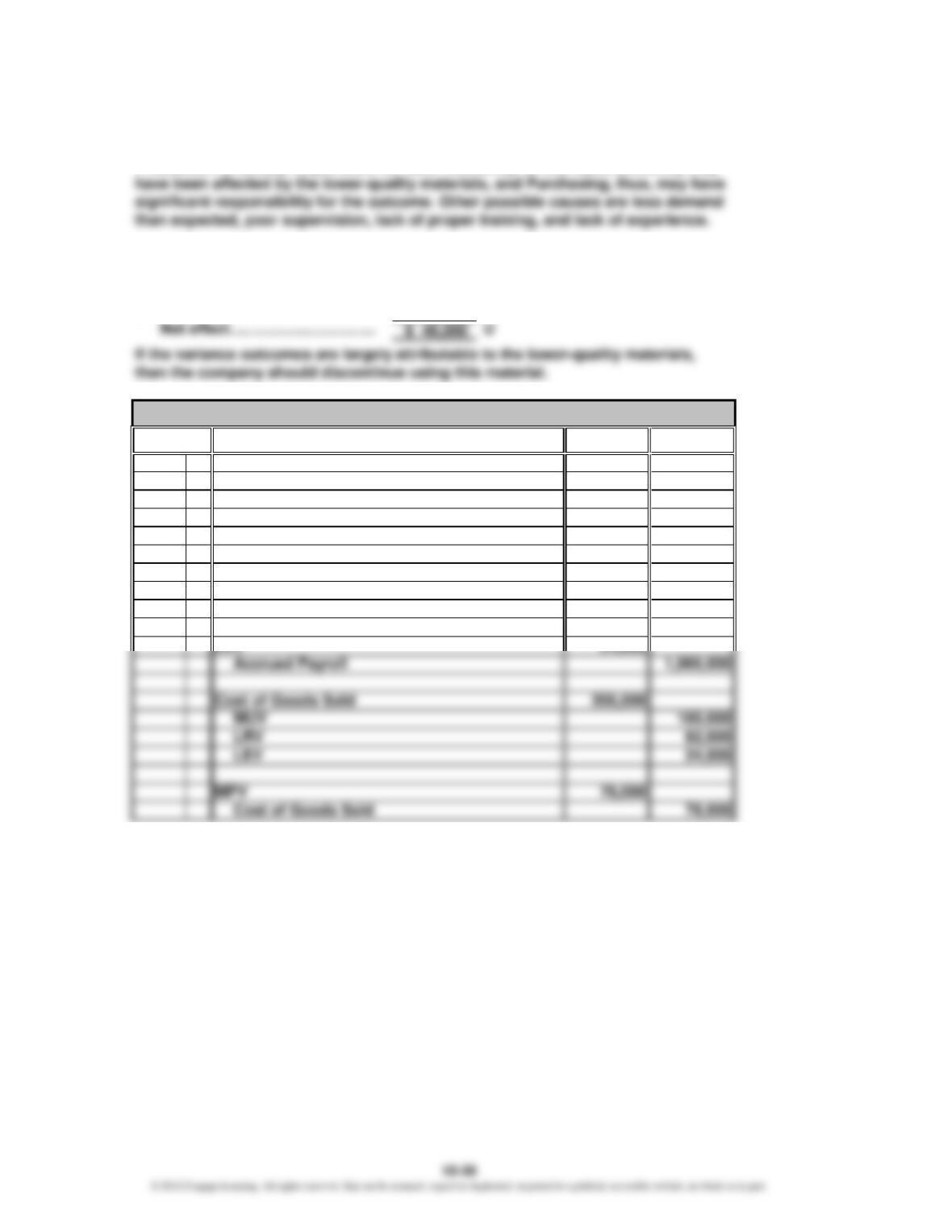
4.
Debit Credit
Materials 1,300,000
MPV 78,000
Accounts Payable 1,222,000
Work in Process 1,500,000
MUV 100,000
Materials 1,600,000
Work in Process 960,000
LRV 82,000
Accrued Payroll 1,066,000
Cost of Goods Sold 206,000
Journal
Date
Account & Explanation

CHAPTER 10: Standard Costing and Variance Analysis
P 10-72 ↓ links ↓
change here, please ↓
1. Standard Fixed Overhead Rate = $2,160,000/(120,000 units × 5 DLH) 2,160,000 /120,000 × 5 = 3.60 Normal vol. 120,000
= $3.60 per DLH Std. labor hrs. for each unit 5
Standard Variable Overhead Rate = $1,440,000/(120,000 units × 5 DLH) 1,440,000 /120,000 × 5 = 2.40 Fixed overhead 2,160,000
= $2.40 per DLH Variable overhead 1,440,000
2. Fixed: 118,600 × 5 × $3.60 = $2,134,800 118,600 × 5 × 3.60 = 2,134,800 Act. prodn. (units) 118,600
Variable: 118,600 × 5 × $2.40 = $1,423,200 118,600 × 5 × 2.40 = 1,423,200
= $15,600 U Act. fixed overhead 2,150,400
=
3. Fixed overhead analysis:
2,150,400 – 2,160,000 = (9,600) F Spending
2,160,000 – 2,134,800 = 25,200 U Volume
The spending variance is the difference between planned and actual costs. Each
item’s variance should be analyzed to see if these costs can be reduced. The
volume variance is the incorrect prediction of volume, or alternatively, it is a signal
of the loss or gain that occurred because of producing at a level different from the
expected level.
4. Variable overhead analysis: ↓ links ↓
2.40 × 592,300 =
1,422,800 – 1,421,520 = 1,280 U Spending
The variable overhead spending variance is the difference between the actual
variable overhead costs and the budgeted costs for the actual hours used. The
variable overhead efficiency variance is the savings or extra cost attributable to
the efficiency of labor usage.
Spending
$1,280 U
$1,423,200
$1,422,800
1,421,520
Budgeted VOH
Applied VOH
Actual FOH
$2,150,400
Budgeted FOH
$2,160,000
Applied FOH
$2,134,800
$9,600 F
Spending
Volume
$25,200 U
Actual VOH
CHAPTER 10 Standard Costing and Variance Analysis
P 10-73
1. Variable overhead variances: ↓ links ↓ links ↓
change here, please ↓
Actual VOH: Fixed OH 6
Budgeted VOH: 40,000 U Spending Variable OH 10
10 × 82,000 = 820,000 Hrs. reqd. per unit 1.6
Applied VOH: 20,000 U Efficiency Act. Prodn 50,000
2. Fixed overhead variances:
Actual VOH:
Budgeted VOH: (20,000) F Spending
6 × 1.60 × 60,000 = 576,000
$20,000 F Applied VOH: 96,000 U Volume
Spending 6 × 1.60 × 50,000 = 480,000
Volume
$20,000 U
556,000
$96,000 U
860,000
Actual VOH
Budgeted VOH
$10 × 82,000 hrs.
Applied VOH
$10 × 80,000 hrs.
$800,000
$556,000
Actual VOH
Budgeted VOH
$6 × 1.6 hrs. ×
60,000 units
$576,000
Applied VOH
$6 × 1.6 hrs. ×
50,000 units
$480,000
$860,000
$40,000 U
$820,000

CHAPTER 10: Standard Costing and Variance Analysis
P 10-74 ↓ links ↓
change here, please ↓
1. Standard Fixed Overhead Rate = $1,286,400/(120,000 units × 4 DLH) 1,286,400 / 120,000 × 4 Normal vol. 120,000
= $2.68 per direct labor hour = 2.68 Std. labor hrs. for each unit 4
Standard Variable Overhead Rate = $888,000/(120,000 units × 4 DLH) 888,000 / 120,000 × 4 Fixed overhead 1,286,400
= $1.85 per direct labor hour = 1.85 Variable overhead 888,000
3. Fixed overhead analysis:
1,300,000 – 1,286,400 = 13,600 U Spending
1,286,400 – 1,275,680 = 10,720 U Volume
The spending variance is the difference between planned and actual costs. Each
item’s variance should be analyzed to see if these costs can be reduced. The
volume variance is the incorrect prediction of volume, or alternatively, it is a signal
of the loss or gain that occurred because of producing at a level different from the
expected level. If practical volume is used to compute the fixed overhead rate, it is a
Actual VOH
$24,395 U
Applied VOH
hours
Spending
Spending
Applied FOH
$1,275,680
Actual FOH
$1,300,000
$13,600 U
Budgeted FOH
$1,286,400
$10,720 U
Volume
CHAPTER 10 Standard Costing and Variance Analysis
P 10-75
1. The budgeted overhead costs are broken down into fixed and variable costs by
change here, please ↓
the high-low method: ↓ links ↓ standard overhead per DLH 18
Standard VOH Rate = 540,000 – 396,000 = 144,000 Budgeted overhead costs 396,000
30,000 – 18,000 = 12,000 Std. DLH 18,000
= $144,000/12,000 hours 144,000 /12,000 = 12 Budgeted overhead costs 540,000
= $12 per hour Std. DLH 30,000
FOH Rate = Total Rate – VOH Rate Actual production 100,000
=$18 – $12 18 – 12 = 6 Fixed overhead volume variance 20,000
=$6 Variable overhead efficiency variance 18,000
Actual fixed overhead costs 200,000
2. Budgeted Fixed Overhead =
Y2 – VX2Actual variable overhead costs 310,000
=$540,000 – $12(30,000) 540,000 – 12 × 30,000
= = 180,000
FOH Spending Variance = Actual FOH – Budgeted FOH
Change in Cost
Change in Activity
$180,000
CHAPTER 10: Standard Costing and Variance Analysis
P 10-76
1.
change here, please ↓
Actual Pairs of shoes to be produced & sold 55,000
Costs Costs* Standard cost per unit:
Direct materials 775,000
2. a. FOH variances: Direct labor 590,000
Spending Variance
=Actual FOH – Budgeted FOH 180,000 – 165,000 = 15,000 U Variable overhead 310,000
=$180,000 – $165,000
=$15,000 U Act. DLH worked 180,000
Volume Variance
=Budgeted FOH – (FOH Rate × SH) Act. Hrs.> Std. hrs. by 63,000
=$165,000 – ($2.50 × 60,000) 165,000 – 2.50 × 60,000 = 15,000 U 5%
=$15,000 U 15,000
b. VOH variances:
Variable OH Rate
=$300,000/60,000 hours 300,000 / 60,000 = 5.00
=$5.00 per hour
Spending Variance
=Actual VOH – (SVOR × AH)
=$310,000 – ($5.00 × 63,000) 310,000 – 5.00 × 63,000 = (5,000) F
=$5,000 F
Efficiency Variance
=(AH – SH)SVOR 63,000 – 60,000 × 5.00 = 15,000 U
=(63,000 – 60,000)$5.00
=$15,000 U
Budgeted
Variance
Shumaker Company
Performance Report
CHAPTER 10 Standard Costing and Variance Analysis
Case 10-77
1. By using a standard costing system, Crunchy Chips can increase control
of its manufacturing inputs. By developing price and quantity standards
for each input, management can compute price and usage variances for
each input. Since a standard costing system provides more information,
2. The engineering standards are ideal standards. The president’s concern
is probably reflecting doubt that the labor standards can be achieved. If
pressure is applied to workers to achieve perfection standards, the
outcome is likely to be unsatisfactory. Workers may become frustrated
CASES
CHAPTER 10: Standard Costing and Variance Analysis
change here, please ↓
Case 10-77 (Concluded) ↓ links ↓ one box holds (bags) 15
3. Standard cost sheet (for one box of chips): 15.9375
@
0.238 = 3.7931 Raw potato pieces are sold at 0.16
Direct materials: 49.50
@
0.04 = 1.9800 Potato cost per pound 0.245
Potatoes (15.9375* lbs. @ $0.238)…………..………………….………………….………………….…………………...…………….
$3.7931 15
@
0.11 = 1.6500 Each potato averages (oz.) 4.25
Cooking oil (49.5 oz. @ $0.04)……………………………………………………………………………….
1.9800 1
@
0.52 = 0.5200 potatoes requ. per bag 16 Oz.
Bags (15 @ $0.11)………………………………………………………………………………..………………………………..
1.6500 it actually has 16.3
Boxes (1 @ $0.52)…………………………………………………………………………………………….…………..
0.5200 $7.9431 * 15 × 4 × 4.25 / 16 = 15.9375 4 Oz.
Direct labor:** Finished chip inspection 12,000
Potato inspection (0.006 hr. @ $15.20)……………………………………..……………………………………..…………………………………..…………..
$0.0912 0.006
@
15.20 = 0.0912 Frying monitor 6,300
Chip inspection (0.0225 hr. @ $10.30)……………………………………..……………………………………..…………………………………..……………
0.2318 0.0225
@
10.30 = 0.2318 Boxing 16,600
Frying monitor (0.0118 hr. @ $14.00)……………………………………..……………………………………..…………………………………..……………
0.1652 0.0118
@
14.00 = 0.1652 Machine operators 6,300
Boxing (0.0311 hr. @ $11.00)……………………………………..……………………………………..…………………………………..……………
0.3421 0.0311
@
11.00 = 0.3421 If the hrs. allowed are higher by: 10%
Machine operators (0.0118 hr. @ $13.00)……………………………………..……………………………………..…………………………………..……………
0.1534 $ 0.9837 0.0118
@
13.00 = 0.1534 Raw potato inspectors 15.20
Variable overhead ($0.9837 × 1.16)………………………………..……………………………………..……………………..
1.1411 0.9837 × 1.16 = 1.1411 Finished chip inspectors 10.3
Fixed overhead (0.9837 × $1.9671)***……………………………………..…………………………………..………………..
1.9350 0.9837 × 1.9671 = 1.9350 Frying monitor 14
Direct materials………………………………………………………………………………………
7.9431 Boxing 11
Cost per box…………………………………………………………..……..……………………………..……………………………………..………
$12.0029 a16 × 4.25 ÷ 4 = 17 Machine operators 13
Cost per bag $12.0029/15 bags………………………………………………………………………………………………………………….
$ 0.8002 12.0029 / 15 = 0.8002 variable overhead (DL) 116%
** Number of boxes per year = 8,800,000/15 = 586,667 586,667 Fixed O/H 1,135,216
Hours/box:
** /15 = 586,667 If prodn. Per yr.(mn. Bags) was 9,500,000
Potato inspection:
** 3,200 × 1.1 / 586,667 = 0.0060
Chip inspection:
** 12,000 × 1.1 / 586,667 = 0.0225
Frying monitor:
** 6,300 × 1.1 / 586,667 = 0.0118
Boxing:
577104.33 ** 16,600 × 1.1 / 586,667 = 0.0311
Machine operators:
** 6,300 × 1.1 / 586,667 = 0.0118
1,135,216
9,500,000
6,300 × 1.1/586,667 = 0.0118
3,200 × 1.1/586,667 = 0.0060
12,000 × 1.1/586,667 = 0.0225
6,300 × 1.1/586,667 = 0.0118
16,600 × 1.1/586,667 = 0.0311
8,800,000
CHAPTER 10 Standard Costing and Variance Analysis
Case 10-78
1. Pat’s decision was wrong and not in the best interests of the company.
His concern for his bonus and promotion was apparently more important
assessment of personal risk was probably a significant input to the
decision to buy the inferior component. All too often, individuals decide to
chances of getting caught. This obviously should not be a factor. What is
2. The use of standards to evaluate performance and assess rewards
apparently was influential in Pat’s decision. He clearly had a desire to
receive his annual bonus and wanted to present an impressive
performance profile so that he could secure a position at division
headquarters. Perhaps altering the factors used for evaluating and
rewarding performance and increasing the tenure of managers may
decrease this type of behavior. Or perhaps we ought to spend more time
emphasizing ethical behavior—maybe the problem isn’t so much the
systems we use for evaluating and rewarding performance but rather the
lack of commitment to ethical decision making.
3. Purchasing agents have ethical responsibilities similar to accountants.
Integrity is a universally desirable characteristic. Pat and other purchasing
agents should refrain from engaging in any activity that would prejudice
be well advised to adopt a set of ethical standards. All employees should
understand that certain behaviors are unacceptable.
4. Answers will vary.
CHAPTER 10: Standard Costing and Variance Analysis
Case 10-79 ↓ links ↓ Supervision 500,000
1. Fixed Overhead Rate = $2,400,000/600,000 hours* 2,400,000 / 600,000 = 4.00 Building lease 800,000
2. Athens plant: Practical capacity 300,000
Budgeted FOH 4 × 600,000 = 2,400,000 U Little Rock units 240,000
actual FOH costs ########
2,500,000 – 2,400,000 = 100,000 U Spending Std. DLH allowed 2
2,400,000 – 2,400,000 = 0 Volume Athens units 300,000
No. of plants 10
Little Rock plant: No. of supervisors 10
4 × 480,000 = 1,920,000 U Supervisor’s salary 50,000
2,500,000 – 2,400,000 = 100,000 U Spending
2,400,000 – 1,920,000 = 480,000 U Volume
The spending variance is almost certainly caused by supervisor salaries
(e.g., an unexpected midyear increase due to union pressures). It is unlikely
that the lease payments or depreciation would be greater than budgeted.
Changing the terms on a 10-year lease in the first year would be unusual (unless
there is some sort of special clause permitting increased payments for something
like unexpected inflation). Also, the depreciation should be on target (unless
more equipment was purchased or the depreciation budget was set before the practical Little Rock DLH
price of the equipment was known with certainty). capacity – units × allowed
The volume variance is easy to explain. The Little Rock plant produced less than 300,000 – 240,000 × 2 =
expected, and so there was an unused capacity cost:
$2,400,000
$480,000 U
Volume
Applied FOH
$4 × 480,000 hours
$1,920,000
Volume
$2,500,000
Actual FOH
$2,500,000
$2,400,000
$0
Applied FOH
$2,400,000
$4 × 600,000 hours
Actual FOH
$100,000 U
Spending
$100,000 U
Spending
Budgeted FOH

CHAPTER 10 Standard Costing and Variance Analysis
Case 10-79 (Concluded) ↓ links ↓ (links to previous)
3. It appears that the 120,000-hour unused capacity (60,000 subassemblies) 300,000 – 240,000 = 60,000 Supervision 500,000
is permanent for the Little Rock plant. This plant has 10 supervisors, each Building lease 800,000
making $50,000. Supervision is a step-cost driven by the number of 50,000 × 2 = 100,000 Equip. depreciation 1,100,000
production lines. Unused capacity of 120,000 hours means that two lines Total Budgeted FOH 2,400,000
can be shut down, saving the salaries of two supervisors ($100,000 at the
original salary level). The equipment for the two lines is owned. If it could be Practical capacity 300,000
sold, then the money could be reinvested and the depreciation charge
would be reduced by 20% (2 lines shut down out of 10). There is no Little Rock units 240,000
way to directly reduce the lease payments for the building. Perhaps the
company could use the space to establish production lines for a different actual FOH costs 2,500,000
product. Or perhaps the space could be subleased. Another possibility is Std. DLH allowed 2
to keep the supervisors and equipment and try to fill the unused capacity Athens units 300,000
with special orders for the subassembly below the regular selling No. of plants 10
price from a market not normally served. If the selling price is sufficient to
cover the variable costs and cover at least the salaries and depreciation No. of supervisors 10
for the two lines, then the special order option may be a possibility. This
option, however, is fraught with risks (e.g., the risk of finding enough Supervisor’s salary 50,000
orders to justify keeping the supervisors and equipment, the risk of
alienating regular customers who pay full price, and the risk of violating
the resource usage model in answering this question (see Chapter 3)].
4. For each plant, the standard fixed overhead rate is $4 per direct labor
hour. Since each subassembly should use 2 hours, the fixed overhead ↓ links ↓
cost per unit is $8, regardless of where they are produced. Should they 4 × 2 = 8
differ? Some may argue that the rate for the Little Rock plant needs to be
recalculated. For example, one possibility is to use expected actual
capacity, instead of practical capacity. In this case, the Little Rock plant
would have a fixed overhead rate of $2,400,000/480,000 hours = $5 per 2,400,000 /480,000 = 5
hour and a cost per subassembly of $10. The question is: Should the 5 × 2 = 10
subassemblies be charged for the cost of the unused capacity? ABC
suggests a negative response. Products should be charged for the
resources they use, and the cost of unused capacity should be reported
this unused capacity.