11-1
CHAPTER 11
RISK-ADJUSTED EXPECTED RATES OF RETURN AND
THE DIVIDENDS VALUATION APPROACH
Solutions to Questions, Exercises, Problems, and Teaching Notes to Cases
11.1 The Dividends-Based Valuation Approach. [LO4] The theory behind the
11.2 Valuation Approach Equivalence. [LO2] Conceptually, students should
understand that the dividends valuation approach yields equivalent value
12. At a conceptual level, dividends valuation and free cash flows to equity
valuation are two sides to the same equation. The dividends approach is based on
11.3 The Risk-Return Trade-off. [LO3] Analysts and investors use risk-adjusted
expected rates of return as discount rates in valuation to capture the effects of the
11.4 The Components of the CAPM. [LO3] The CAPM computes expected rates of
return using the following model (described in the chapter):
[
]
[
]
[
]
{
}
ER = ER +βER ER
⎡⎤ ×−
Chapter 11
11-2
© 2018 Cengage Learning®. May not be scanned, copied or duplicated, or posted to a publicly accessible website, in whole or in part.
average level of systematic risk. The product of the second and third components
represents the amount of return the investor should expect for bearing the level of
systematic risk in an investment in Firm j relative to the average level of
systematic risk in the market.
11.5 Nondiversifiable and Diversifiable Risk Factors. [LO3] Firm-specific factors
that increase the firm’s nondiversifiable risk (systematic risk) include the firm’s
exposure to economywide risk factors such as interest rate changes, inflation,
foreign exchange rate changes, and cyclicality. Firm-specific exposure to such
11.6 Debt and the Weighted-Average Cost of Capital. [LO3] Investors typically
accept a lower risk-adjusted rate of return on debt capital than on equity capital
because debt is typically less risky because fixed claims bear less residual risk
11.7 Firms That Do Not Pay Periodic Dividends. [LO4] The dividends valuation
approach is applicable to firms that do not pay periodic (quarterly or annual)
11.8 Dividend Policy Irrelevance. [LO4] The chapter relies on the seminal work of
Modigliani and Miller (1961), with which most students will be familiar, to assert
Chapter 11
11-3
© 2018 Cengage Learning®. May not be scanned, copied or duplicated, or posted to a publicly accessible website, in whole or in part.
the firm retains the capital to earn the same return. You should anticipate
students’ questions about conditions under which the irrelevance theorem may not
hold, including when dividend payments signal information to shareholders or
when a non-dividend-paying firm becomes increasingly vulnerable to agency
problems because managers are underinvesting the firm’s resources.
11.9 Measuring Value-Relevant Dividends. [LO5] The chapter emphasizes an “all-
inclusive” measurement approach to “value-relevant” dividends. For dividends-
11.10 Calculating Required Rates of Return on Equity Capital across Different
Industries. [LO3]
a. Utilities versus Petroleum and Natural Gas 0.75 versus 1.45
Both industries are engaged in the production of energy. The typical utility
firm is highly leveraged, which would increase systematic risk, but the typical
Chapter 11
Risk-Adjusted Expected Rates of Return and the Dividends Valuation Approach
11-4
Banking (Depository Institutions) versus Financial Trading (Security
and Commodity Brokers) 0.88 versus 1.13
and fees from arranging deals and placements of capital.
b. and c. Assuming that the risk-free rate of return is 4.0% and the market risk
premium is 5.0%, we compute the following required rates of return for each
industry. Using the perpetuity-with-growth model and assuming 3.0% long-
run growth, we compute the following values of a stream of $1 dividends for
the median firm in each industry. These data indicate that differences in
systematic risk can have dramatic effects on valuation.
Industry Median Beta
Expected Return
per CAPM
Perpetuity Value
per $1 of
Dividends
11-5
11.11 Calculating the Cost of Capital. [LO3] (dollar amounts in millions)
a. Whirlpool: ………………… 3.5% + (2.27 × 5.0%) = 14.85%
IBM: ………………………… 3.5% + (0.78 × 5.0%) = 7.40%
Target: ……………………… 3.5% + (1.20 × 5.0%) = 9.50%
b. Whirlpool IBM Target
regardless of its capital structure.
c. As shown in the chapter, the formula to compute unlevered equity (asset) beta
from a levered equity beta is as follows:
Unlevered Market Beta = Current Levered Market Beta/[1 + (1 – Income Tax
Rate) × (Current Market Value of Debt/Current Market Value of Equity)]
Chapter 11
Risk-Adjusted Expected Rates of Return and the Dividends Valuation Approach
11-6
© 2018 Cengage Learning®. May not be scanned, copied or duplicated, or posted to a publicly accessible website, in whole or in part.
d. The revised equity beta for each company is as follows:
New Levered Market Beta = Unlevered Market Beta × [1 + (1 – Income Tax
Rate) × (New Market Value of Debt/New Market Value of Equity)]
Whirlpool:
X = 1.445[1 + (1 – .35) × (.75/.25)]
X = 2.818
X = 1.269
X = 1.519
The revised equity betas for IBM and Target increase significantly because of
the much higher proportion of debt in the new capital structure. Note that the
revised equity beta for Whirlpool increases, but less so than for the other two
firms because Whirlpool’s new capital structure would add a relatively lower
11-7
11.12 Calculation of Dividends-Based Value. [LOs 3-7]
This problem is a straightforward and comprehensive application of the
techniques of Chapter 11 to Royal Dutch Shell Corporation (Shell; ticker:
RDSA.AS).
Required
(0.0705 – 0.03)
Present Value of Continuing Value = $302,205 = $424,850 × 0.7113
d. Compute the total present value of dividends for Shell as of the beginning of
Year +1. Remember to adjust the present value for midyear discounting.
Chapter 11
Risk-Adjusted Expected Rates of Return and the Dividends Valuation Approach
11-8
11.13 Valuing the Equity of a Privately Held Firm. [LOs 5-7]
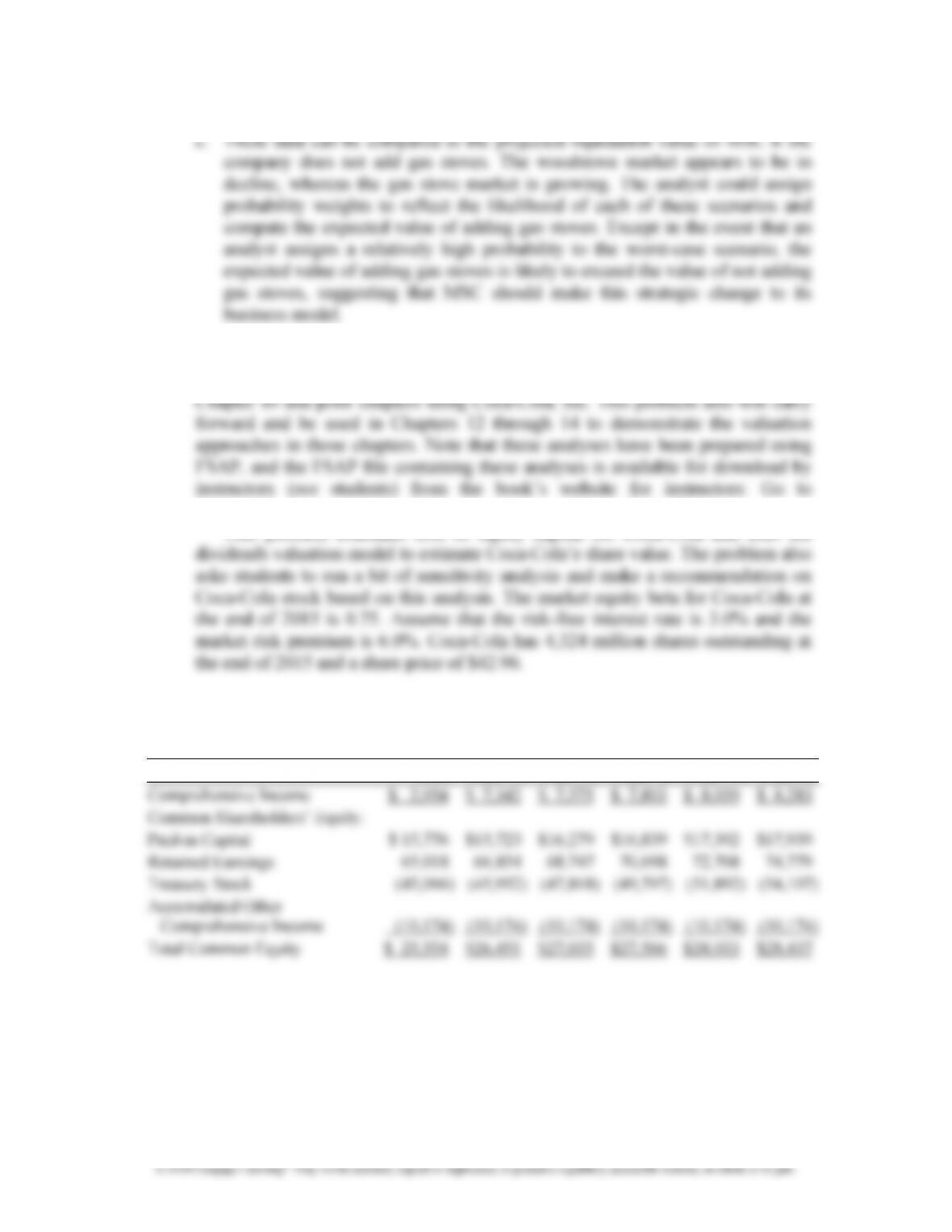
a. Clean surplus accounting applied to MSC each year in each of the three
scenarios reveals that MSC is not paying any dividends.
Year 8 Year 9 Year 10 Year 11 Year 12
Best-Case Scenario:
– Ending Common
Equity (687,423) (761,860) (834,759)
(944,116) (1,094,093)
= Total Dividends 0000 0
Worst-Case Scenario:
Net Income $ 128,263 $ 18,796 $ (39,902) $ (58,316) $ (77,156)
Chapter 11
Risk-Adjusted Expected Rates of Return and the Dividends Valuation Approach
11-9
© 2018 Cengage Learning®. May not be scanned, copied or duplicated, or posted to a publicly accessible website, in whole or in part.
c. These data can be compared to the projected liquidation value of MSC if the
company does not add gas stoves. The woodstove market appears to be in
decline, whereas the gas stove market is growing. The analyst could assign
probability weights to reflect the likelihood of each of these scenarios and
compute the expected value of adding gas stoves. Except in the event that an
analyst assigns a relatively high probability to the worst-case scenario, the
expected value of adding gas stoves is likely to exceed the value of not adding
gas stoves, suggesting that MSC should make this strategic change to its
business model.
11.14 Dividends-Based Valuation of Common Equity. [LOs 3-7] This is an
extensive, integrated problem that connects the topics of Chapter 11 to those of
instructor’s resources page at www.cengage.com/accounting/wahlen.
This problem estimates cost of equity capital for Coca-Cola and uses the
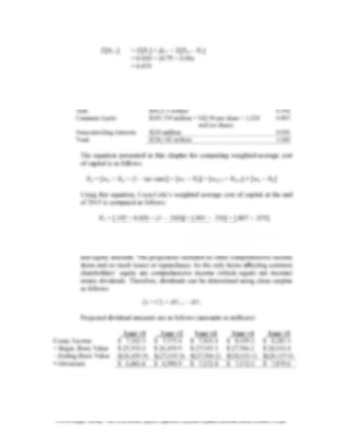
The case provides the following forecast data (amounts in millions):
Actual Projected
2015 Year +1 Year +2 Year +3 Year +4 Year +5
Required
a. Following the CAPM, Coca-Cola faces a required rate of return on equity
capital of 7.5% at the end of 2015. This rate is computed as follows:
Chapter 11
Risk-Adjusted Expected Rates of Return and the Dividends Valuation Approach
11-10
© 2018 Cengage Learning®. May not be scanned, copied or duplicated, or posted to a publicly accessible website, in whole or in part.
E[RCC] = E[RF] + βCC × E[RM – RF]
= 0.030 + (0.75 × 0.06)
= 0.075
b. Coca-Cola’s capital structure at the end of 2015 consists of the following
amounts and proportions:
Amount Weight
= .00292 + .00014 +.06053 = 0.06358 = 6.358%.
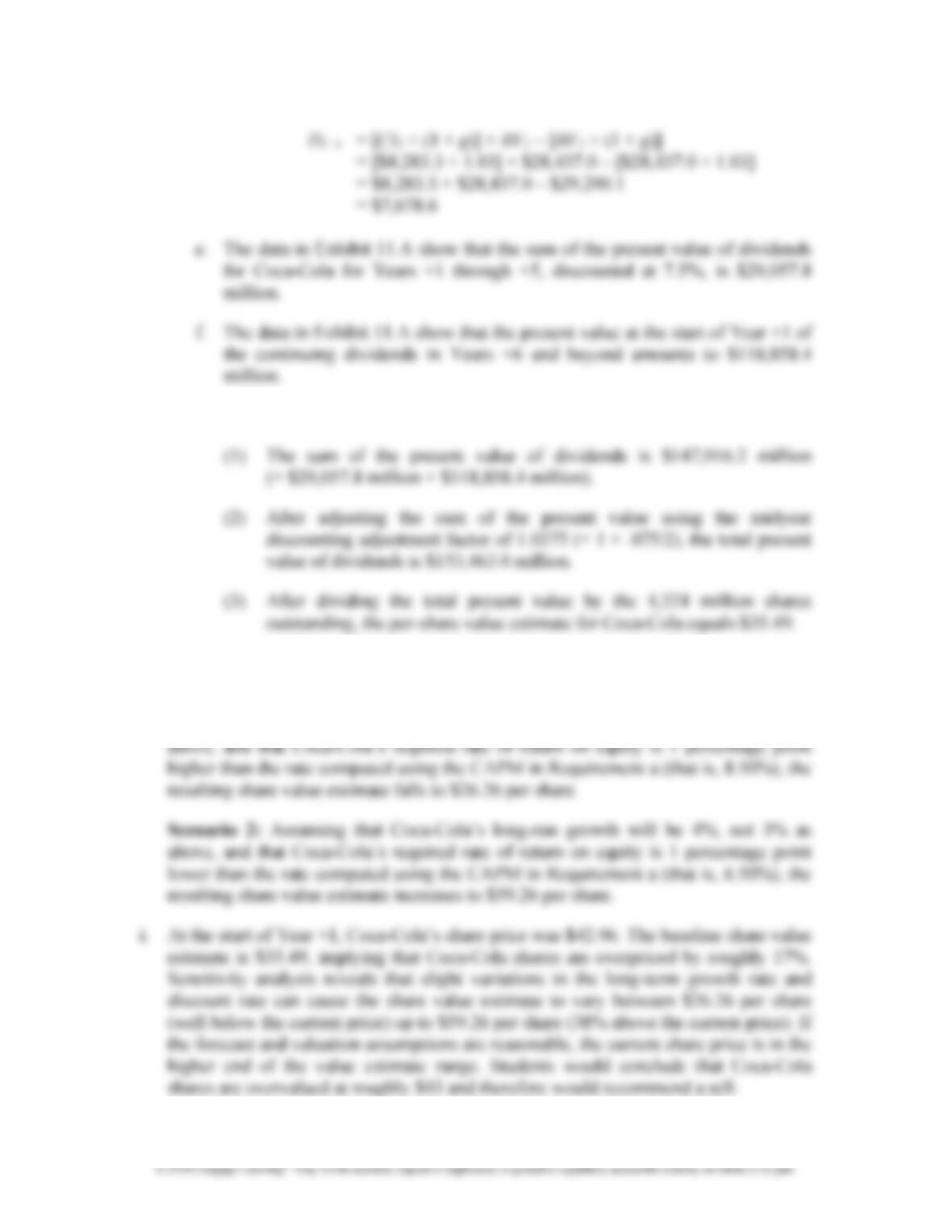
c. The projected value-relevant dividends for Coca-Cola for Years +1 through
+5 are straightforward to derive using the projected comprehensive income
d. Using the approach shown in the chapter to project the continuing dividend in
Year +6 and assuming a steady-state long-run growth rate of 3% results in the
following dividend amount (in millions) in Year +6:
Chapter 11
Risk-Adjusted Expected Rates of Return and the Dividends Valuation Approach
11-11
© 2018 Cengage Learning®. May not be scanned, copied or duplicated, or posted to a publicly accessible website, in whole or in part.
DT+1 = [CIT × (1 + g)] + BVT – [BVT × (1 + g)]
= [$8,283.3 × 1.03] + $28,437.0 – [$28,437.0 × 1.03]
= $8,283.3 + $28,437.0 – $29,290.1
= $7,678.6
e. The data in Exhibit 11.A show that the sum of the present value of dividends
for Coca-Cola for Years +1 through +5, discounted at 7.5%, is $29,057.8
million.
f. The data in Exhibit 11.A show that the present value at the start of Year +1 of
the continuing dividends in Years +6 and beyond amounts to $118,858.4
million.
g. The data in Exhibit 11.A show the following computations:
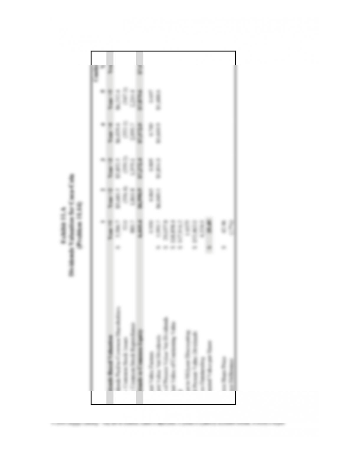
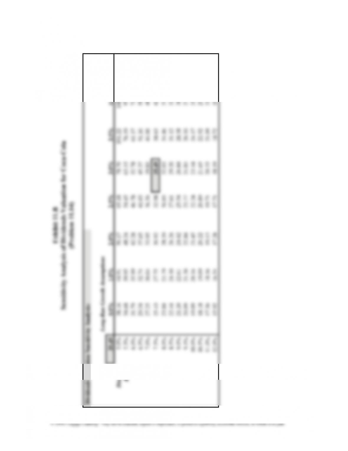
h. The data in Exhibit 11.B show the results of various sensitivity analysis scenarios,
varying discount rates and growth rates.
Scenario 1: Assuming that Coca-Cola’s long-run growth will be 2%, not 3% as
11-12
Chapter 11
Risk-Adjusted Expected Rates of Return and the Dividends Valuation Approach
Dividends Valuation for Coca-Cola
Dividends-Based Valuation Year +1 Year +2 Year +3 Year +4 Year +5 Year +6
Dividends Paid to Common Shareholders $ 5,506.7 $5,681.5 $5,852.5 $6,029.4 $6,212.4
Less: Common Stock Issues 53.0 (556.4) (559.2) (553.1) (547.3)
Plus: Common Stock Repurchases 885.7 1,865.8 1,979.1 2,095.7 2,214.4
Dividends to Common Equity 6,445.4 $6,990.9 $7,272.4 $7,572.0 $7,879.6 $7,678.6
Present Value Factors 0.930 0.865 0.805 0.749 0.697
Present Value Net Dividends $ 5,995.7 $6,049.5 $5,854.0 $5,669.9 $5,488.6
Sum of Present Value Net Dividends $ 29,057.8
Present Value of Continuing Value $ 118,858.4
Total $ 147,916.2
Adjust to Midyear Discounting 1.0375
Total Present Value Dividends $ 153,463.0
Shares Outstanding 4,324.0
Estimated Value per Share $ 35.49
Current Share Price $ 42.96
Percent Difference (17%)
11-13
Chapter 11
Risk-Adjusted Expected Rates of Return and the Dividends Valuation Approach
Sensitivity Analysis of Dividends Valuation for Coca-Cola
Dividends Valuation Sensitivity Analysis:
Long-Run Growth Assumptions
35.49 0.0% 1.0% 2.0% 2.5% 3.0% 3.5% 4.0% 5.0%
Discount 5.0% 38.16 44.91 56.17 65.18 78.70 101.22 146.26
Rates: 5.5% 34.68 39.95 48.24 54.45 63.15 76.19 97.93 271.87
6.0% 31.79 35.99 42.28 46.78 52.78 61.17 73.76 136.72
6.5% 29.34 32.74 37.65 41.03 45.37 51.16 59.26 91.67
7.0% 27.25 30.04 33.95 36.56 39.81 44.00 49.59 69.13
7.5% 25.43 27.75 30.92 32.98 35.49 38.63 42.68 55.61
8.0% 23.84 25.79 28.39 30.05 32.03 34.46 37.49 46.59
8.5% 22.44 24.10 26.26 27.61 29.20 31.12 33.46 40.15
9.0% 21.20 22.61 24.42 25.54 26.84 28.38 30.23 35.31
9.5% 20.09 21.30 22.84 23.77 24.85 26.10 27.59 31.55
10.0% 19.09 20.14 21.45 22.24 23.14 24.17 25.39 28.54
10.5% 18.18 19.09 20.22 20.89 21.65 22.52 23.52 26.07
11.0% 17.36 18.16 19.13 19.71 20.35 21.09 21.92 24.01
12.0% 15.92 16.54 17.28 17.71 18.19 18.72 19.32 20.78
Chapter 11
Risk-Adjusted Expected Rates of Return and the Dividends Valuation Approach
11-14
Integrative Case 11.1: Walmart
Dividends-Based Valuation of Walmart’s Common Equity. This is an extensive
integrated case that connects all of the topics of the text. This portion of the case connects
for instructors: Go to instructor’s resources page at www.cengage.com/accounting/wahlen.
Integrative Case 10.1 projected financial statements for Walmart for Years +1
through +5. This portion of the Integrative Case applies the techniques in Chapter 11 to
The case provides the following forecast data:
Actual Projected
2015 Year +1 Year +2 Year +3 Year +4 Year +5
Required
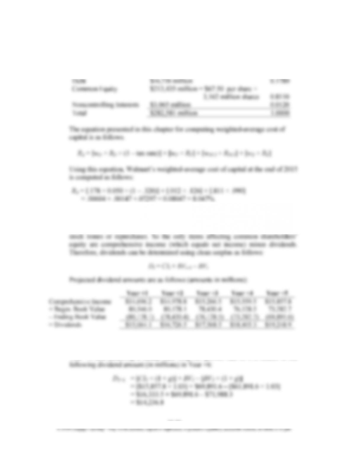
a. Following the CAPM, Walmart faces a required rate of return on equity capital of
9.0 percent at the end of 2015. This rate is computed as follows:
Chapter 11
Risk-Adjusted Expected Rates of Return and the Dividends Valuation Approach
11-15
b. Walmart’s capital structure at the end of 2015 consists of the following amounts
and proportions:
Amount Wei
g
h
t
c. It is straightforward to derive the projected value-relevant dividends for Walmart
for Years +1 through +5 using the projected comprehensive income and equity
amounts. The projections included no other comprehensive income items and no
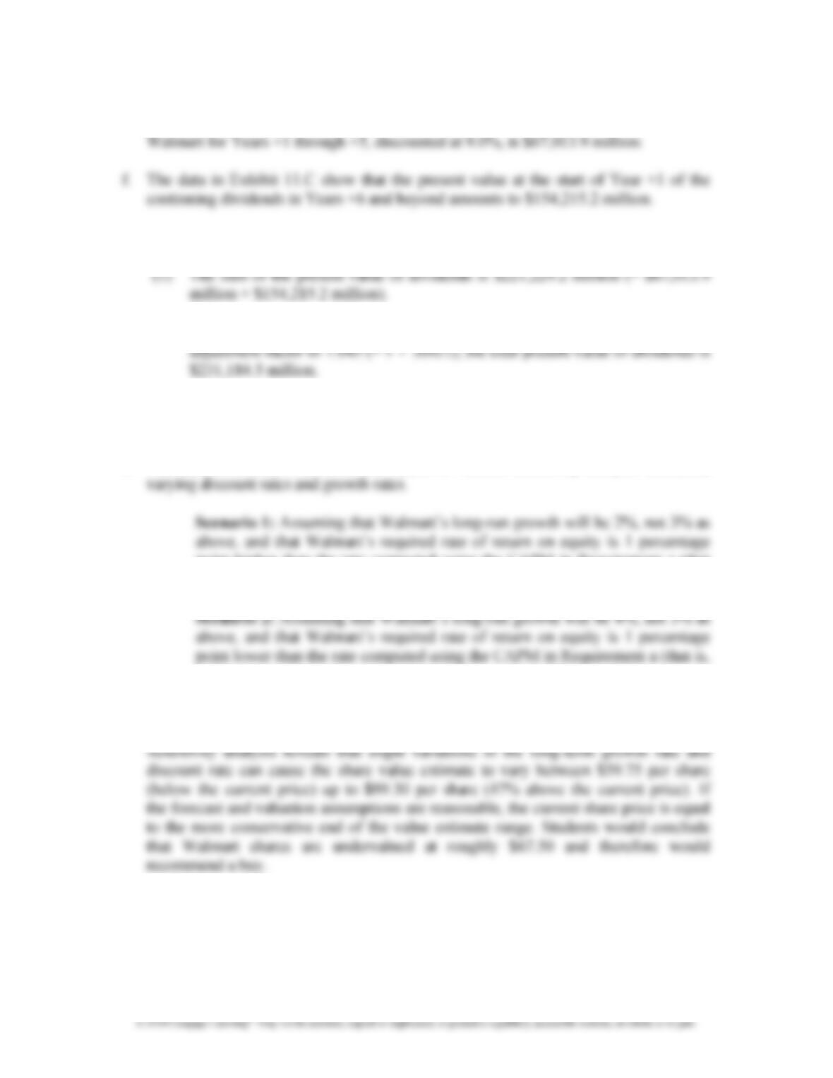
d. Using the approach shown in the chapter to project the continuing dividend in
Year +6 and assuming a steady-state long-run growth rate of 3% results in the
Chapter 11
Risk-Adjusted Expected Rates of Return and the Dividends Valuation Approach
11-16
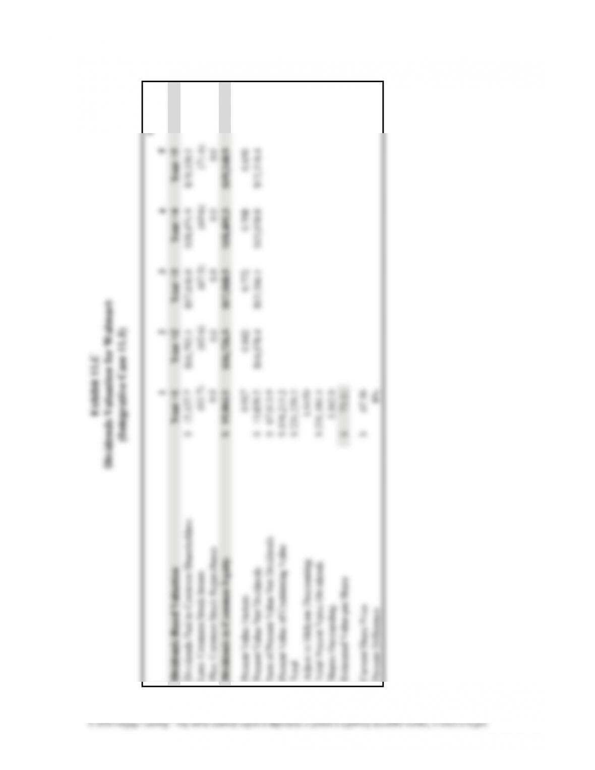
e. The data in Exhibit 11.C show that the sum of the present value of dividends for
g. The data in Exhibit 11.C show the following computations:
(2) After adjusting the sum of the present value using the midyear discounting
(3) After dividing the total present value by the 3,162 million shares outstanding,
the per-share value estimate for Walmart equals $73.11.
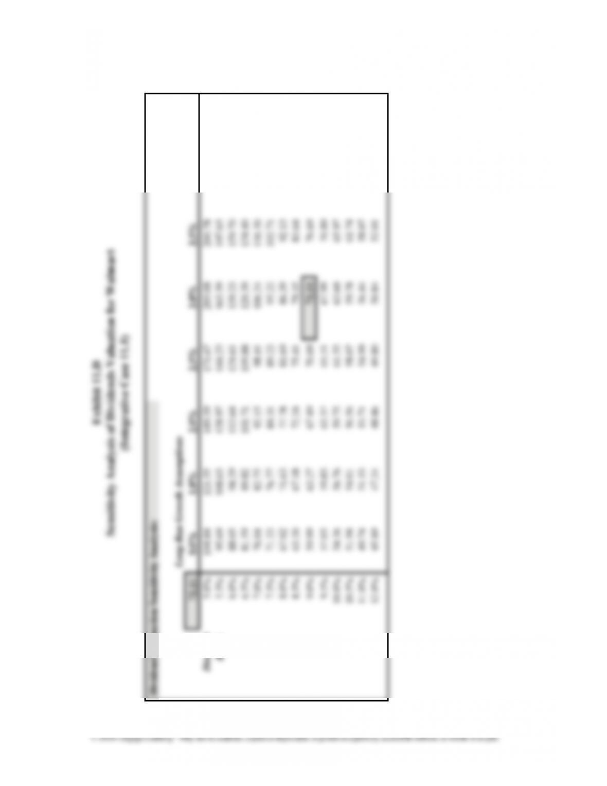
h. The data in Exhibit 11.D show the results of various sensitivity analysis scenarios,
point higher than the rate computed using the CAPM in Requirement a (that
is, 10.0%), the resulting share value estimate falls to $59.75 per share.
8.0%), the resulting share value estimate increases to $99.30 per share.
i. At the start of Year +1, Walmart’s share price was $67.50. The baseline share value
estimate is $73.11, implying that Walmart shares are underpriced by roughly 8%.
11-17
Chapter 11
Risk-Adjusted Expected Rates of Return and the Dividends Valuation Approach
11-18
Chapter 11
Risk-Adjusted Expected Rates of Return and the Dividends Valuation Approach
Sensitivity Analysis of Dividends Valuation for Walmart
Dividends Valuation Sensitivity Analysis:
Long-Run Growth Assumptions
73.11 0.0% 1.0% 2.0% 2.5% 3.0% 3.5% 4.0% 5.0%
Discount 5.0% 104.84 121.55 149.39 171.67 205.08 260.78 372.16
Rates: 5.5% 95.69 108.63 128.97 144.23 165.59 197.63 251.02 678.20
6.0% 88.05 98.29 113.64 124.61 139.23 159.70 190.41 343.96
6.5% 81.59 89.82 101.71 109.88 120.39 134.40 154.01 232.48
7.0% 76.04 82.75 92.15 98.41 106.24 116.30 129.72 176.69
7.5% 71.23 76.77 84.31 89.22 95.22 102.71 112.35 143.18
8.0% 67.02 71.63 77.78 81.69 86.39 92.13 99.30 120.81
8.5% 63.30 67.18 72.24 75.41 79.15 83.64 89.13 104.81
9.0% 59.99 63.27 67.49 70.09 73.11 76.69 80.99 92.79
9.5% 57.03 59.83 63.37 65.51 67.99 70.89 74.31 83.43
10.0% 54.36 56.76 59.75 61.55 63.60 65.97 68.73 75.92
10.5% 51.94 54.01 56.56 58.07 59.78 61.74 64.00 69.76
11.0% 49.74 51.53 53.71 54.99 56.44 58.07 59.94 64.62
12.0% 45.89 47.24 48.86 49.80 50.84 52.01 53.32 56.50