978-1337127363 Chapter 9 Solution Manual Part 2

subject Type Homework Help
subject Pages 7
subject Words 1248
subject Authors Christopher M. Snyder, Walter Nicholson

Unlock document.

This document is partially blurred.
Unlock all pages and 1 million more documents.
Get Access
page-pf1
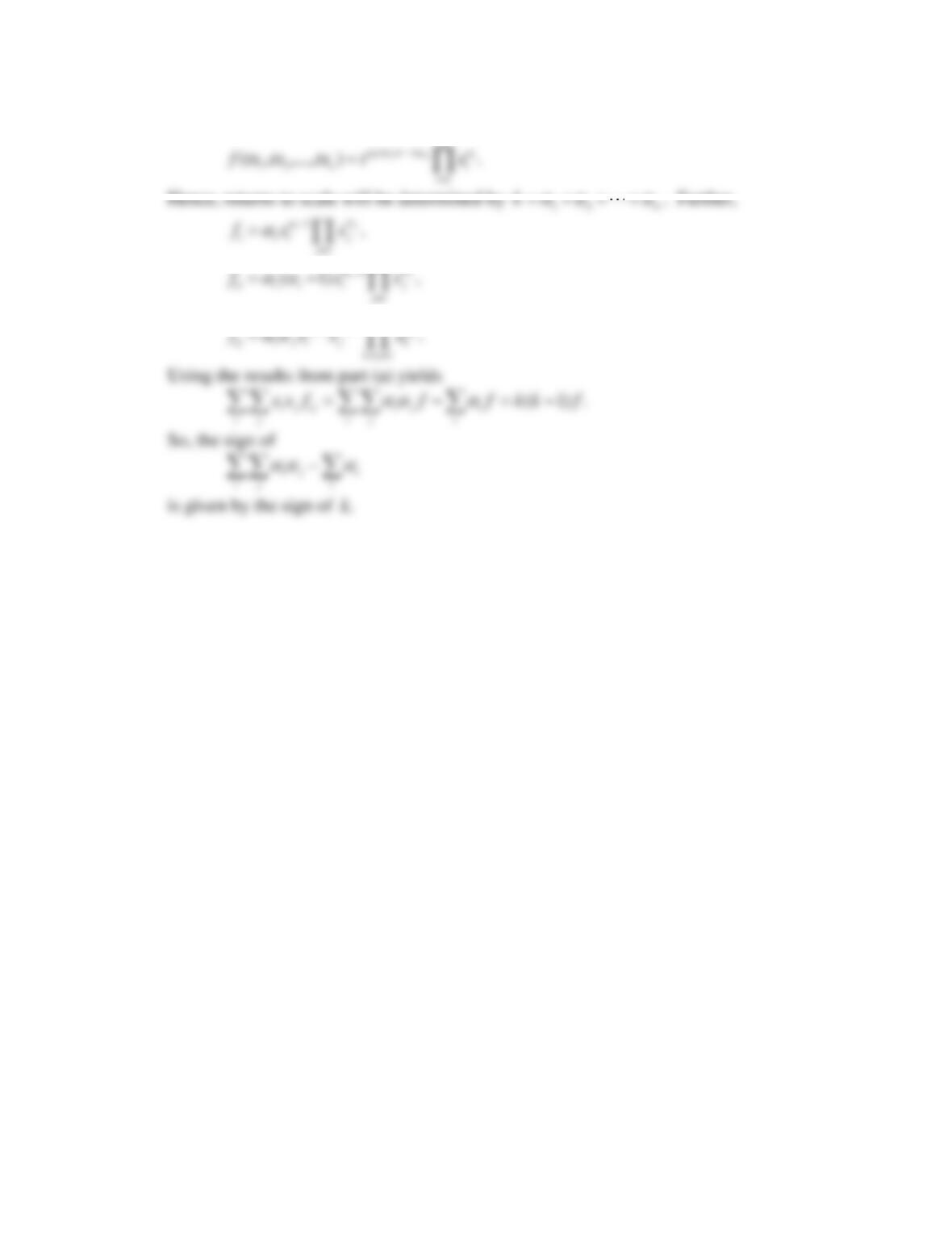
9.6 a. We have
1
.
1
k
11
1
q1
MP = = +
k l k
k
=
qk
q
= k





Similar manipulations yield
.
1
l
q
MP = l



b. Using the results from part (a),
1
.
k
l
MP l
RTS = =
MP k



Inverting,
1
1,
lRTS
k
implying
1
1,
kRTS
l
in turn implying
1
ln ln .
1
kRTS
l



From Equation 9.32,
ln 1
= = .
ln 1
d k l
d RTS
c. Computing elasticities,
,
1,
1( )
qk
q k q
e = = =
k q k + l k



11
.
11
q, l q
=
el+ k l + l k

 


Putting these over a common denominator yields
,,
1,
q k q l
e e =
which shows
constant returns to scale.
d. The result follows directly from part (a) since
page-pf2
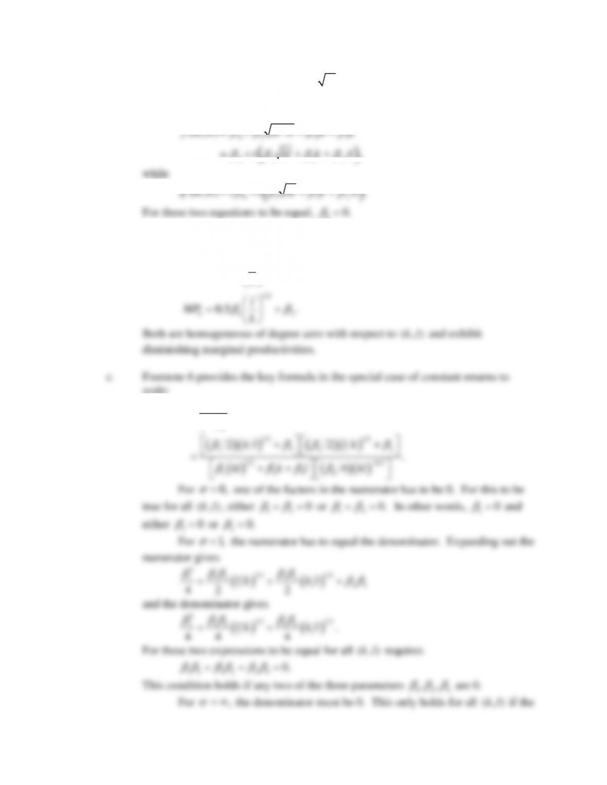
9.7 Given production function
0 1 2 3
( , ) .f k l = kl k l
a. For constant returns to scale,
( , ) ( , ).f tk tl = tf k l
But
0 1 2 3
0 1 2 3
( , )
,
f tk tl = tk tl tk tl
t kl k tl
while
0 1 2 3
( , ) .tf tk tl t t kl k tl
For these two equations to be equal,
00.
b. Assume
00
to ensure constant returns to scale. Then
0.5
13
0.5
12
0.5 ,
0.5 .
l
k
k
MP l
l
MP k










Both are homogeneous of degree zero with respect to
( , )kl
and exhibit
diminishing marginal productivities.
c Footnote 6 provides the key formula in the special case of constant returns to
scale:
1 2 1 2
1 3 1 2
1 2 1 2
1 2 3 1
22
.
4
lk
kl
ff
ff
k l l k
kl k l kl


For
0,
one of the factors in the numerator has to be 0. For this to be
true for all
( , )kl
, either
13
0


or
12
0.


In other words,
10
and
either
30
or
20.
For
1,
the numerator has to equal the denominator. Expanding out the
numerator gives
21 2 1 2
13
1 1 2 23
4 2 2
l k k l


and the denominator gives
21 2 1 2
13
1 1 2 .
4 4 4
l k k l


For these two expressions to be equal for all
( , )kl
requires
1 3 1 2 2 3 0.
This condition holds if any two of the three parameters
1 2 3
,,
are 0.
For
,

the denominator must be 0. This only holds for all
( , )kl
if the
page-pf3
second factor is 0, that is,
12
14 0.kl
For this condition to hold for all
( , )kl
requires
10.
9.8 Because
( , )q f k l
exhibits constant returns to scale, it is homogeneous of degree 1. In
this special case, Euler’s theorem (Equation 2.109) states
( , ) .
kl
q f k l f k f l
Rearranging,
.
lk
qk
ff
ll



a. If
( , ) ( , ),f tk tl tf k l
then
,1
1
( , )
lim ( , )
( , )
lim ( , )
1.
qt t
t
f tk tl t
et f tk tl
f k l
f k l

page-pf4
2 1 1
,1
2 3 1 1
1
11
(1 )
lim
lim 2
2
1
21
2 2 .
qt t
t
t k l t
etq
t
q t k l q
qk l
qq
q















Hence,
,1
qt
e
for
0.5,q
and
,1
qt
e
for
0.5.q
d. The intuitive reason for the changing scale elasticity is that this function has an
upper bound of
1q
and gains from increasing the inputs decline as
q
9.10 Returns to scale and substitution
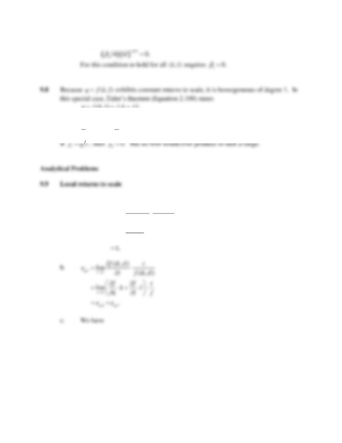
a. Let
denote the elasticity of substitution and
RTS
the marginal rate of technical
substitution associated with
.F
Then
1
1.
l l l
k k k
F f f f
RTS RTS
F f f f
Because
f
is homogeneous of degree 1, it is homothetic, and so
RTS
is a
function only of the input ratio: that is,
( ).RTS B k l
Hence,
( ),k l b RTS
where
1.bB
We have
()
,
d k l RTS
d RTS k l
RTS
b RTS kl
RTS
d k l RTS
kl
d RTS
page-pf5
.
kl
kl
ff
ff


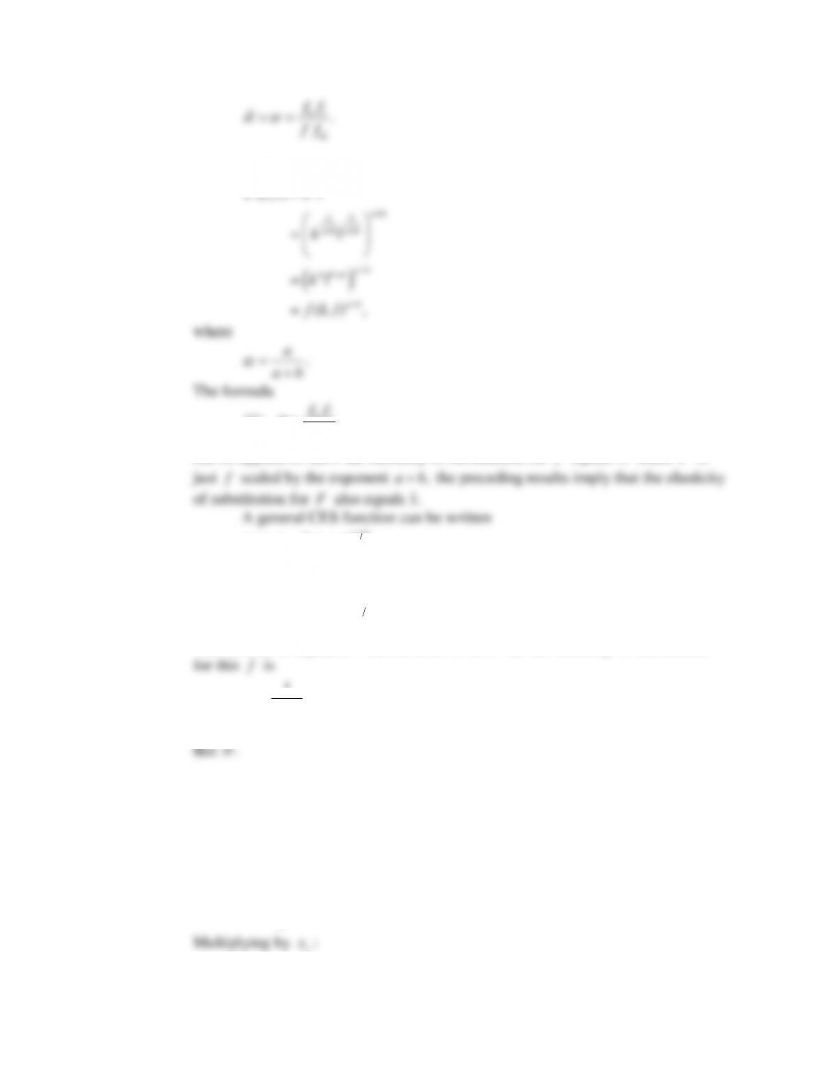
b. A general CobbDouglas for arbitrary returns to scale can be written
1
( , )
( , ) ,
ab
ab
ab
a b a b
ab
ab
F k l k l
kl
kl
f k l





where
.
a
ab
The formula
(1) σkl
kl
ff
ff
can be applied to show the elasticity of substitution for
f
equals 1. Since
F
is
γρ
ρρ
γ
( , )
( , ) ,
F k l k l
f k l

where
1
( , ) .f k l k l


The formula in Equation 1 can be used to show that the elasticity of substitution
Hence, the elasticity of substitution for general CES function
F
is the same as
9.11 More on Euler’s theorem
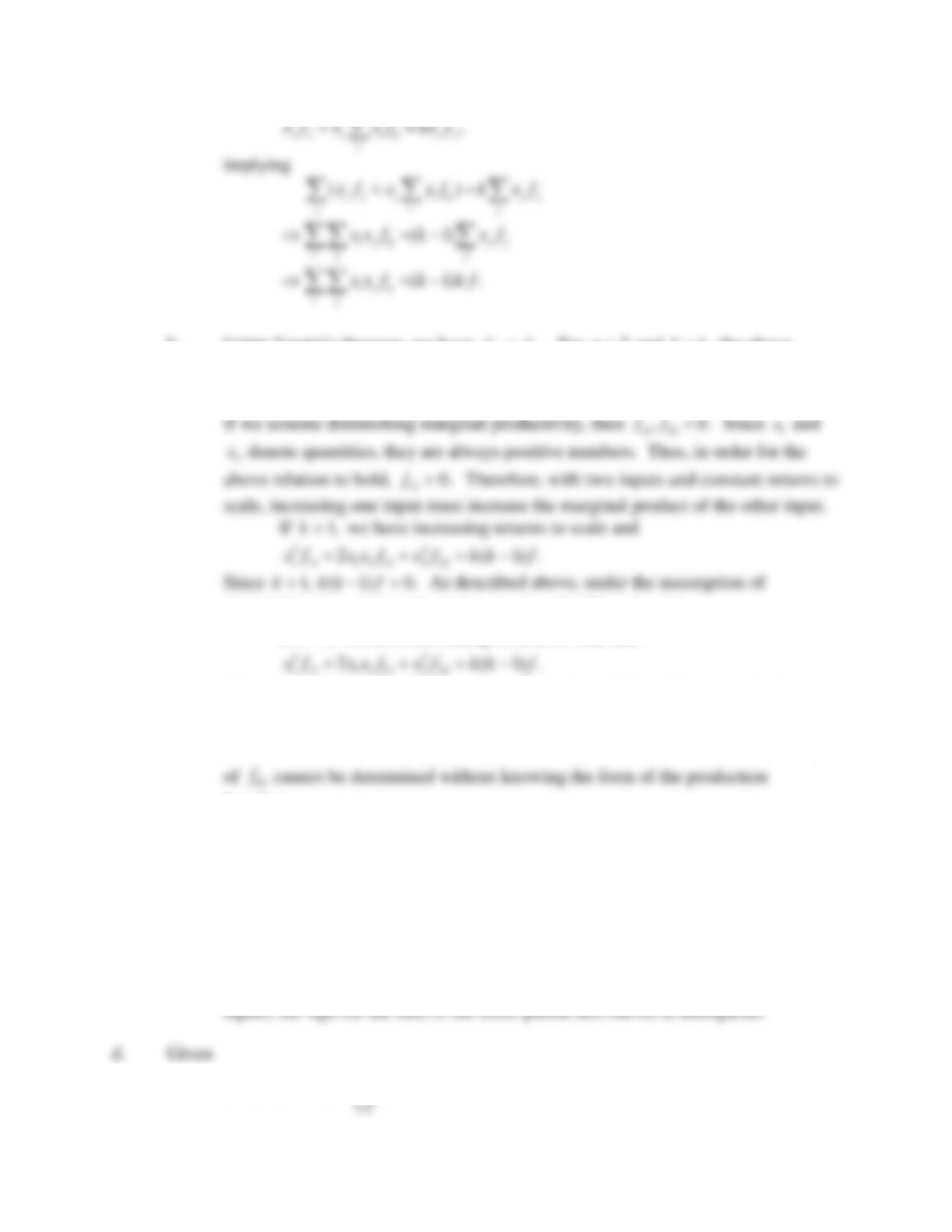
a. By Euler’s theorem:
.
ii
i
x f kf
Differentiating with respect to
:
j
x
.
j i ij j
i
f x f kf
page-pf6
,
j j j i ij j j
i
x f x x f kx f
implying
()
( 1)
( 1) .
j j j i ij j j
j i j
i j ij j j
i j j
i j ij
ij
x f x x f k x f
x x f k x f
x x f k k f


b. Using Young’s theorem, we have
12 21.ff
For
2n
and
1,k
the above
expression becomes
22
1 11 1 2 12 2 22
2 0.x f x x f x f
diminishing marginal productivity,
11 22
, 0.ff
Thus,
12 0.f
If
1,k
we have decreasing returns to scale and
22
1 11 1 2 12 2 22
2 ( 1) .x f x x f x f k k f
Since
1,k
( 1) 0.k k f
Under the assumption of diminishing marginal
productivity,
11 22
, 0.ff
Therefore, the left-hand side of the expression must be
negative, and this could happen if
12 0f
or
12 0.f
Thus, in this case, the sign
12
function.
c. Under the assumption of diminishing marginal productivity,
0
ii
f
for
1,..., .in
Thus, we cannot infer the sign of any one of the cross-partial derivatives. But, for
1,k
we know that
0
i j ij
ij
x x f

for the expression in part (a) to hold. Therefore, at least one cross-partial
derivative must be positive. For the case of
1,k
like in the case of only two
12 1
( , ,..., ) .
i
n
ni
i
f x x x x
page-pf7
we have
12
12 1
( , ,..., ) .
ni
n
ni
i
f tx tx tx t x
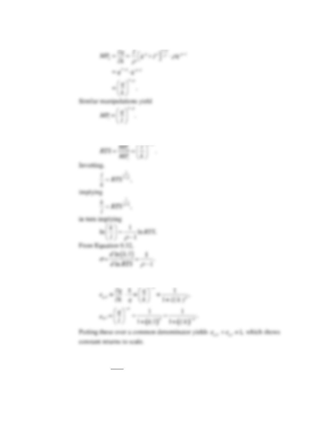
Hence, returns to scale will be determined by
12 n
k
. Further,
1
2
1
1
,
( 1) ,
.
j
i
j
i
j
ik
i i i j
ji
ii i i i j
ji
ij i j i j k
k j i
f x x
f x x
f x x x





Using the results from part (a) yields
( 1) .
i j i j i j i
i j i j i
x x f f f k k f
So, the sign of
i j i
i j i
is given by the sign of
.k

Trusted by Thousands of
Students

Here are what students say about us.

Copyright ©2022 All rights reserved. | CoursePaper is not sponsored or endorsed by any college or university.