13 112
0 2 3
1
32
23
32
32
1
2
3
22
1.
33
F
F
rF
rF
x F dx r dr
r
FF
Analytical Problems
12
1
()
() ()
1
(1 )( )
(1 )
.
Uw
rw Uw
w
w
w
The reciprocal,
1 ( ),rw
is linear in
w
since it is of the form
,a bw
and
1.
()
w
rw
b. When
0
and
1
1,
0
1
( ) .
w
w
rw
Thus,
()rw
is a constant as required if
.
d. Let
1
( ) .r w A
Then
( ) ( ).U w AU w
Solving this differential equation demonstrates
( ) .
Aw
U w ke
2
2
22
() 1
()
( 2 ).
w
Uw
w
ww
Thus, we have a quadratic utility function.
a. A high value for
1R
implies a low elasticity of substitution between states of
the world. A very risk-averse individual is not willing to make trades away from
the certainty line except at very favorable terms.
b.
1R
implies the individual is risk-neutral. The elasticity of substitution between
wealth in various states of the world is infinite. Indifference curves are linear with
slopes of
1.
If
,R
the individual has an infinite relative risk-aversion
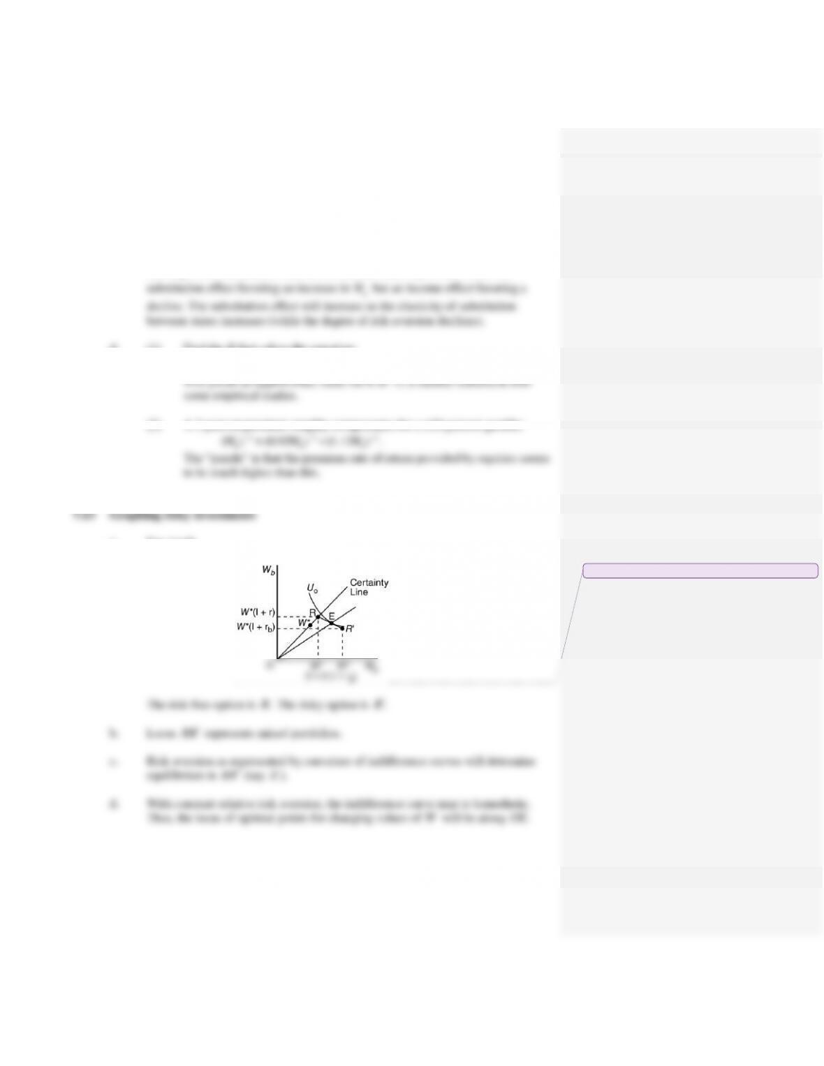
parameter. His or her indifference curves are L-shaped implying an unwillingness
to trade away from the certainty line at any price.
c. A rise in
b
p
rotates the budget constraint counterclockwise about the
g
W
intercept. Both substitution and income effects cause
b
W
to fall. There is a
d. (1) Find the R that solves the equation:
0 0 0
( ) 0.5(1.055 ) 0.5(0.955 ) .
R R R
W W W
(2) A 2 percent premium roughly compensates for a 10 percent gamble:
3 3 3
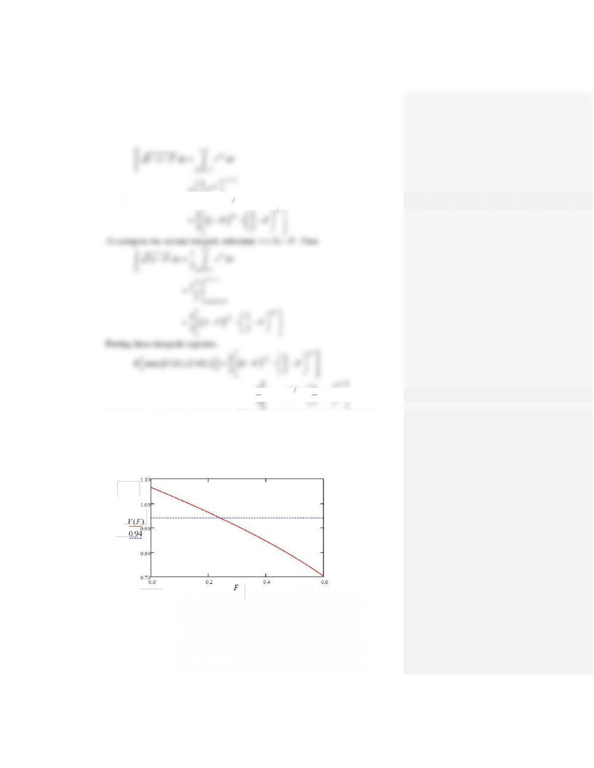
a. See graph.
Commented [C1]: COMP: Please change r, rb, I, rg to r, rb, I, rg.
7.14 The portfolio problem with a Normally distributed asset
From Example 7.3,
2
( ) .
2
Ww
A
E U W
For the portfolio allocation, we are looking to allocate
k
to the risky asset and
0–Wk
to
the risk-free one. Since the risky asset
r
is normally distributed with the distribution
( , )
rr
N
and final wealth is given by
0(1 ) ( )
ff
W W r k r r
(see Equation 7.48), final wealth is distributed as
0
( ) (1 ) ( )
f r f
E W W r k r
Expected utility is given by
22
0
( ) (1 ) ( ) .
2
f r f r
A
E U W W r k r k
Hence,
rf
ur
0,
r
k
20,
r
k
0.
k
A
less to be invested in it.
Behavioral Problem
Scenario 2
Gamble
Expected wealth
C
2,000 1 2 (1,000 0) 1,500
D
2,000 500 1,500
a. Scenarios (
A
)–(
D
) provide the same expected wealth—$1,500—so a risk-
neutral Stan should be indifferent among them.
the safe option
B
in Scenario 1 and
D
in Scenario 2.
c. It is natural to suppose subjects are risk averse, so more should choose option
D
subjects. Scenario 1 involves gains, so Pete behaves as predicted by
may be preferred.
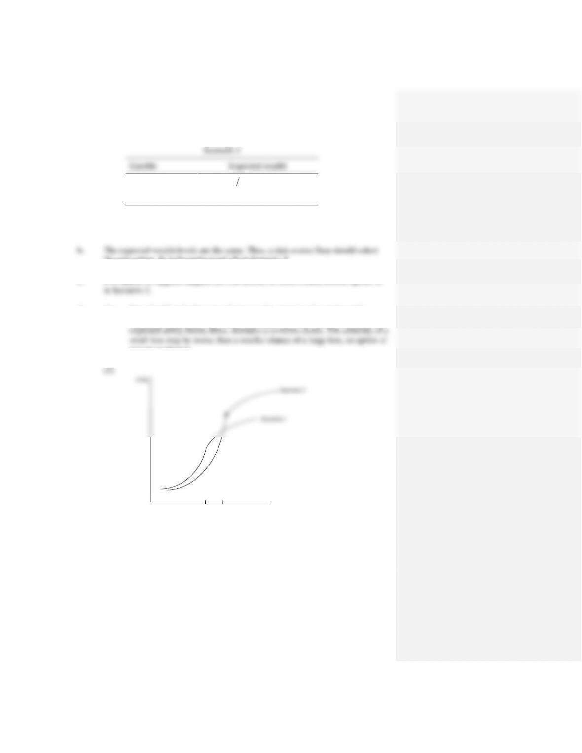
The utility curve has to shift because of the kink at the anchor point.
Prospect Pete’s curve changes from convex to concave at the anchor point;
Standard Stan’s is linear or concave everywhere, so doesn’t have to shift.
Utility
Scenario 1
•
Wealth
1,000
Scenario 2
•
2,000