
Most of the problems in this chapter focus on illustrating the concept of risk aversion. They
assume that individuals have concave utility of wealth functions and therefore dislike variance in
their wealth. For some of these problems (especially the later ones), students will need to review
the material on mathematical statistics in Chapter 2.
Comments on Problems
7.1 This problem reverses the risk-aversion logic to show that observed behavior can be used
to place bounds on subjective probability estimates.
presented here.
7.3 This is a nice, homey problem about diversification. The problem can be done
graphically, but instructors could introduce variances into the problem if desired.
7.4 This problem is a graphical introduction to the economics of health insurance that
examines cost-sharing provisions. Health insurance is discussed in more detail in Chapter
18.
7.5 This problem provides some simple numerical calculations involving risk aversion and
insurance when utility is logarithmic.
7.6 This is a rather difficult problem as written. It can be simplified by using a particular
utility function (e.g.,
( ) lnU W W
). With the logarithmic utility function, one cannot use
the Taylor approximation until after differentiation, however. If the approximation is
applied before differentiation, concavity (and risk aversion) is lost. This problem can,
with specific numbers, also be done graphically, if desired. The notion that fines are more
effective can be contrasted with the criminologist’s view that apprehension of law–
provisions can affect diversification.
CHAPTER 7:
Uncertainty

7.9 This is a new problem on diversification, here applied to investing in financial assets. The
problem illustrates a case in which it is optimal to diversify into an asset with obviously
lower expected returns. The problem shows that diversification can be beneficial with
Analytical Problems
special cases of the HARA function.
7.12 More on the CRRA function. This problem stresses the close connection between the
7.13 Graphing risky investments. This problem provides an illustration of investment theory
in the state preference framework.
7.14 The portfolio problem with a Normally distributed risky asset. This problem shows
how the portfolio problem can be solved explicitly if asset returns are Normal.
behavioral economics, which Kahneman (Nobel Prize winner) and Tversky applied to
explain the results of their lab experiments. Actual experimental results are cited in the
problem.
Solutions

ln 1,100,000 1 ln 900,000 ln 1,000,000 .pp
Solving,
13.9108 13.7102 1 13.8155,pp
implying
2006 0.1053,p
or
0.525.p
7.2 See graph.
7.3 a.
Strategy 1
Outcome
Probability
12 Eggs
0.5
0 Eggs
0.5
Expected value =
0.5 (12) 0.5( 0) 6.
Strategy 2
Outcome
Probability
12 Eggs
0.25
6 Eggs
0.5
0 Eggs
0.25
Expected value =
0.25 (12) 0.5( 6) 0.25(0) 3 3 6.
b.
Commented [C1]: COMP: Please set h as h.
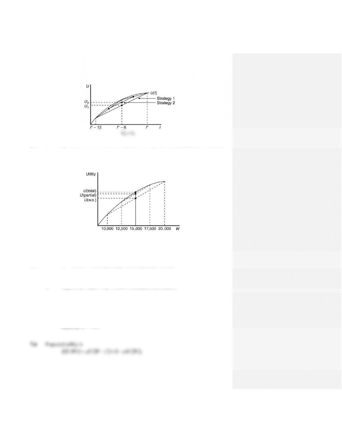
7.4 a. The insurance company has a 50% chance of paying out $10,000. Its cost is thus
$5,000. The consumer has a certain wealth of $15,000 with fair insurance
compared to a 50–50 chance of wealth of $10,000 or $20,000 without insurance.
b. Cost of the policy is
0.5 5,000 2,500
. Hence, wealth is 17,500 with no illness
and 12,500 with the illness.
7.5 a.
no ins[ ( )] 0.75ln 10,000 0.25ln 9,000 9.1840.E U Y
b.
ins[ ( )] ln 9,750 9.1850.E U Y
Insurance is preferable.
c. We have
ln(10,000 ) 9.1840.p
Exponentiating,
9.1840
10,000 9,740,pe
implying
260.p


Calculate
p
when
10W
k
p
0.5
0.0125
1
0.05
2
0.2
Risk premium is higher when the level of initial wealth is lower. The greater the
Calculate
p
when
100W
k
p
0.5
0.00125
1
0.005
2
0.02

implying
0.444.
Plugging
into the utility function yields
*mix[ ( )] 0.5 ln 22,996 0.5 ln 12,780 9.7494.E U Y
This is a slight improvement over the 50–50 mix.
d. If the farmer plants only wheat,
24,000
NR
Y
and
14,000.
R
Y
equal split 1 1 1 1
[ ( )] 12.5 0 8 4.5 2.121,
4 4 4 4
E U W
a
in
A
and
1a
in
B
leads to four possible
outcomes: the assets both turn out to yield a positive return, generating
utility
16 9(1 );aa
they both yield no return, generating utility
0 0;
A
yields a positive return and
B
does not, generating utility
16 4 ;aa
and vice versa, generating utility
9(1 ) 3 1 .aa
Each
11
4 3 1 .
44
aa
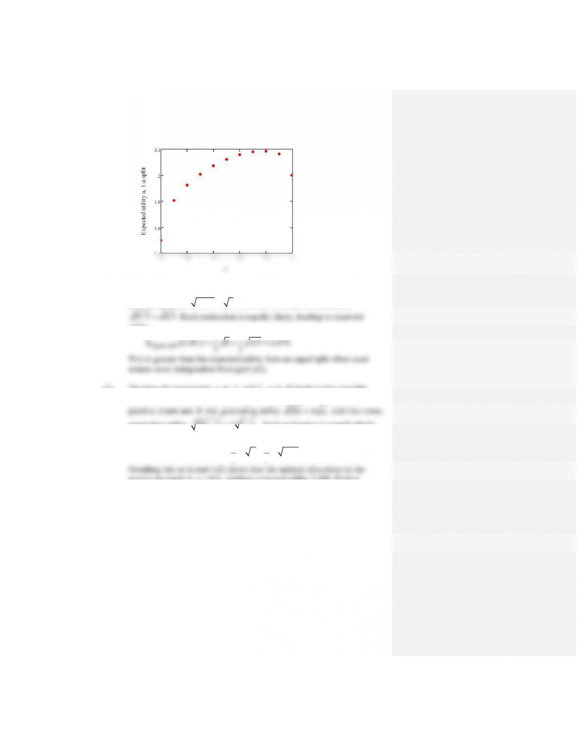
One could try to maximize this with respect to
a
, but it is simpler to graph
it, as below, and see that the maximum is reached, restricting attention to
decimal values of
,a
for
0.8,a
at which point the expected utility is
2.185, higher than from an equal split. While Maria still diversifies, she
b. (1) With perfect negative correlation, and half invested in each asset, there are
only two possible outcomes:
A
has a positive return and
B
nothing,
generating utility
16/ 2 8;
and vice versa, generating utility
9 / 2 4.5.
Each realization is equally likely, leading to expected
utility
equal split 11
[ ( )] 8 4.5 2.475.
22
E U W
This is greater than the expected utility from an equal split when asset
returns were independent from part (a1).
(2) Dividing the investment
a
in
A
and
1a
in
B
leads to two possible
outcomes when there is perfect negative correlation:
A
can yield a
generating utility
9(1 ) 3 1 .aa
Each realization is equally likely,
leading to expected utility
,1 split 11
[ ( )] 4 3 1 .
22
aa
E U W a a
nearest decimal) is
0.6,a
yielding expected utility 2.498. Perfect
negative correlation makes diversification even more appealing.