The problems in this chapter focus mainly on the utility maximization assumption. Relatively
simple computational problems (mainly based on Cobb–Douglas and CES utility functions) are
included. Comparative statics exercises are included in a few problems, but for the most part,
introduction of this material is delayed until Chapters 5 and 6.
Comments on Problems
might be told to find the correct bundle on the original indifference curve first, and then
compute its cost.
4.2 This problem uses the Cobb–Douglas utility function to solve for quantity demanded at
4.3 This problem starts as an unconstrained maximization problem—there is no income
constraint in part (a) on the assumption that this constraint is not limiting. In part (b),
ensure a local maximum.
4.5 This problem is an example of a “fixed proportion” utility function. The problem might
be used to illustrate the notion of perfect complements and the absence of relative price
effects for them. Students may need some help with the min ( ) functional notation by
using illustrative numerical values for v and g and showing what it means to have
“excess” v or g.
4.7 This problem repeats the lessons of the lump-sum principle for the case of a subsidy.
Numerical examples are based on the Cobb–Douglas expenditure function.
CHAPTER 4:
Utility Maximization and Choice
4.8 This problem uses two very simple utility functions to show how all of the major
work through the various possibilities logically.
4.10 Cobb–Douglas utility. This problem provides a simple example of the Cobb–Douglas
expenditure function and seeks to build some intuition about how a good’s relative
importance affects that function.
relatively straightforward but part (d) is computationally difficult. A somewhat different
form for this function is examined in Problem 4.13.
4.12 Stone–Geary utility. This problem introduces a simple two-good Stone–Geary function
4.13 CES indirect utility and expenditure functions. This problem uses a more standard
form for the CES utility function and asks students to delve more deeply into the
4.14 Altruism. This problem shows a simple way in which altruism can be incorporated into
a standard Cobb–Douglas utility function.
Solutions
4.1 a. To find maximum utility given a fixed budget, set up the Lagrangian:
(1.00 0.10 0.25 ).ts t s
L
The first-order conditions are
0.5
0.5
0.10 0,
ds
dt t
dt
L
L
would not be expected to hold for more complicated forms of the utility function.
In part (b),
2/3 1 3
( , ) 20 25 21.5.U f c
This person will need more income to achieve the part (b) utility with the part (a)
prices. Setting the value of indirect utility to the utility level in part (b):
2 3 1 3
2 3 1 3
2 3 1 3
2 3 1 3
21
21.5 33
21(40) (8) .
33
fc
I p p
I
4.3 Given
22
( , ) 20 18 3 .U c b c c b b
a. The first-order conditions are
20 2 0,
18 6 0.
Uc
c
Ub
b
Solving,
*10,c
*3,b
and
*127.U
b. The constraint is
5.bc
Set up the Lagrangian:
22
20 18 3 (5 ).c c b b c b
L
The first-order conditions are
20 2 0,
18 6 0,
5 0.
c
b
c
b
cb
L
L
L
Solving the first two equations yields
3 1.cb
So
3 1 5,bb
implying
*1,b
*4,c
and
*79.U
4.4 Given
2 2 0.5
( , ) ( ) .U x y x y
Note that maximizing
2
U
will also maximize
.U
22(50 3 4 ).x y x y
L
The first-order conditions are
2 3 0,
2 4 0,
50 3 4 0.
x
y
x
y
xy
L
L
L
The first two equations give
4 3.yx
Substituting in budget constraint gives
*6,x
*8,y
*10.U
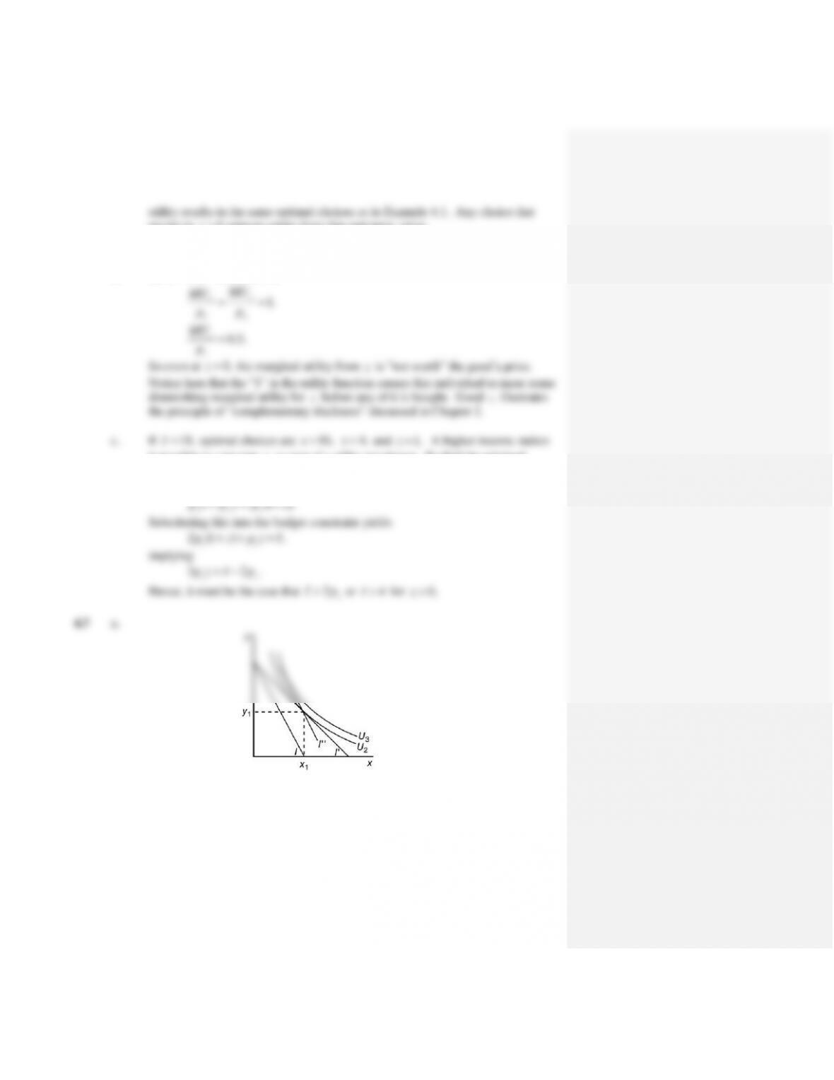
a. No matter what the relative prices are (i.e., the slope of the budget constraint), the
maximum utility intersection will always be at the vertex of an indifference curve
b. Substituting
2gv
into the budget constraint yields
2,
gv
p v p v I
or
.
2gv
I
vpp
Furthermore,
2.
2gv
I
gpp
It is easy to show that these two demand functions are homogeneous of degree
zero in
,
g
p
,
v
p
and
.I
c. Since
2,U g v
indirect utility is
( , , ) .
2
gv
gv
I
V p p I p + p
d. The expenditure function is found by interchanging
()IE
and
V
,
( , , ) (2 ) .
g v g v
E p p V p p V
results in
0z
reduces utility from this optimum, since
0.5 0.5 0.5
(0.9) ((3.6) 1.1 89,) 1.U
which is less than
0().Uz
b. At
4,x
1y
, and
0.z
y
x
MU
MU
it possible to consume
z
as part of a utility maximum. To find the minimal
income at which any (fractional)
z
would be bought, use the fact that this person
will spend equal amounts on
,x
,y
and
(1 )z
with the Cobb–Douglas:
b.
0.5 0.5
( , , ) 2 .
x y x y
E p p U p p U
With
1
x
p
and
4,
y
p
we have
2U
and
8.E
To raise utility to 3 would require
12,E
that is, an income
subsidy of 4.
0.5 0.5
0.5 8 12 2 3.
d.
0.3 0.7
( , , ) 1.84 .
x y x y
E p p U p p U
With
1
x
p
and
4,
y
p
we have
2U
and
9.71.E
Raising
U
to 3 would require extra expenditures of 4.86.
Subsidizing good
x
alone would require a price of
0.26,
x
p
that is, a subsidy of
0.74 per unit. With this low price, the person would choose
11.2,x
so the total
price would have to fall to 0.6 to reach a utility level of 5 with an expenditure of
8. In this case, consumption would be
5, 1.25xy
and the cost of the subsidy