
These problems provide some practice in examining utility functions by looking at
indifference curve maps and at a few functional forms. The primary focus is on
illustrating the notion of quasi-concavity (a diminishing MRS) in various contexts. The
concepts of the budget constraint and utility maximization are not used until the next
chapter.
Comments on Problems
3.1 This problem requires students to graph indifference curves for a variety of
functions, some of which are not quasi-concave.
3.2 This problem introduces the formal definition of quasi-concavity (from Chapter
2) to be applied to the functions studied graphically in Problem 3.1.
3.3 This problem shows that diminishing marginal utility is not required to obtain a
diminishing MRS. All of the functions are monotonic transformations of one
another, so this problem illustrates that diminishing MRS is preserved by
monotonic transformations but diminishing marginal utility is not.
3.4 This problem focuses on whether some simple utility functions exhibit convex
indifference curves.
3.5 This problem is an exploration of the fixed-proportions utility function. The
problem also shows how the goods in such problems can be treated as a
composite commodity.
3.6 This problem asks students to use their imaginations to explain how advertising
slogans might be captured in the form of a utility function.
3.7 This problem shows how utility functions can be inferred from MRS segments. It
is a very simple example of “integrability.”
3.8 This problem offers some practice in deriving utility functions from indifference
curve specifications.
Analytical Problems
CHAPTER 3:
Preferences and Utility

in simple indifference curve analysis.
3.10 Cobb–Douglas utility. This problem provides some exercises with the Cobb–
Douglas function, including how to integrate subsistence levels of consumption
into the functional form.
3.11 Independent marginal utilities. This problem shows how analysis can be
simplified if the cross-partials of the utility function are zero.
3.12 CES utility. This problem shows how distributional weights can be incorporated
into the CES form introduced in the chapter without changing the basic
conclusions about the function.
3.13 The quasi-linear function. This problem provides a brief introduction to the
quasi-linear form, which (in later chapters) will be used to illustrate a number of
interesting outcomes.
3.14 Preference relations. This problem provides a very brief introduction to how
preferences can be treated formally with set-theoretic concepts.
3.15 The benefit function. This problem introduces Luenberger’s notion of reducing
preferences to a cardinal number of replications of a basic bundle of goods.

3.2 Because all of the first-order partials are positive, we must only check the second-
order partials.
b.
, 0, 0.
XX yy xy
U U U
Strictly quasi-concave.
,xy
both of the second-order
partials are ambiguous, and therefore the function is not necessarily
strictly quasi-concave.
e.
, 0, 0.
xx yy xy
U U U
Strictly quasi-concave.
3.3 a.
,
x
Uy
0,
xx
U
,
y
Ux
0,
yy
U
.MRS y x
b.
2
2,
x
U xy
2
2 0,
xx
Uy
2
2,
y
U x y
2
2 0,
yy
Ux
.MRS y x
.MRS y x

are maximum, specifically,
11
k x y
and
22
.k y x
Then
12
( ) 2x x k
and
12
( ) 2 ,y y k
implying
1 2 1 2
x x y y
c. $1.60.
d. $2.10, an increase of 31 percent.
e. Price would increase only to $1.725, an increase of 7.8 percent.
f. Raise prices so that a fully condimented hot dog rises in price to $2.60.
3.6 For all the suggested utility functions, let x represent some other good and the
good in question is represented by the appropriate letter:
a.
( , ) ( , ) for .U x p U x b p b
b. Given
( , ), 0
xc cx
U x c U U
.
c. Given
( , ), ( ,1) ( ,0) ( , 1).U x p U x U x U x p
d.
( , ) ( , ) for U x kk U x dd kk dd
.
e.
responsible responsible
( , ) ( , ) for .U x m U x m m m
Using this formula, yields:
12
48
y
x
Now use the fact that the two points yield equal utility:
Commented [C2]: COMP: Please set all Greek letters in
22
The utility function is of the form
2.U x y
c. Yes, there was a redundancy. We never used the information about the
second MRS. In fact, given that the function is assumed to be Cobb–
Douglas, only the information about the first MRS was needed to get the
ratio of the exponents. Since utility is invariant up to a monotonic
transformation, any Cobb–Douglas for which
2
would yield the
same behavior. For example, if the exponents sum to one, we have
2/3, 1/3
and this function also satisfies the conditions of the
problem.
3.8 a. Exponentiate the function:
.U x y z
b. Move the term in x to the LHS:
22
.U x xy y
Commented [C1]: COMP: Please set all Greek letters in
italic.
italic.
Commented [C3]: COMP: Please set all Greek letters in
italic.

2
2 2 2 .U x y y z z x
Analytical Problems:
3.9 Initial endowments
a.
b. Any trading opportunities that differ from the MRS at
,xy
will provide
the opportunity to raise utility (see figure).
c. A preference for the initial endowment will require that trading
opportunities raise utility substantially. This will be more likely if the
3.10 Cobb–Douglas utility
a.
1
1.
U x x y y
MRS U y x y x
values
x
relatively more highly. Hence,
1MRS
for
.xy
c. The function is homothetic in
0
xx
and
0
yy
, but not in
x
and
.y

, 0.
xx yy
UU
Conversely, the Cobb–Douglas not only has
0
xy
U
and
,0
xx yy
UU
, but also has a diminishing MRS (see Problem 3.10a).
a.
1
1
1,
U x x y
MRS U y y x
so this function is homothetic.
b. If
1,
,MRS
a constant. If
0,
,
y
MRS x
This agrees with Problem 3.10.

d. Since the marginal utility of
x
is a constant at 1 while that of
y
is
decreasing as
y
increases (as it is of the form
1y
), we would expect
consumers to shift more toward
x
when they buy more of both goods. We
explore this in much more detail in the next chapter.
e. Refer to Example 3.4. This function is usually used to describe the
consumption of one commodity with respect to all other commodities. So,
ln y
could represent the commodity of interest, while
x
could represent
all the other goods consumed.
3.14 Preference relations
All of the suggested preference relations are complete, transitive, and continuous.
a. Summation:
contained.
Transitive: If bundle A has more items than B and B has more
items than C, clearly A has more items than C.
Continuous: If bundle A contains more items than bundle B, then
A is preferred to B and any bundle with slightly more items than B
(but fewer than A) is also preferred to B.
the (i + j)th good, then A will be preferred to C because it will
break the tie at the ith good also.

Continuous: Suppose bundle A is preferred to B with the tie break
occurring at the ith good. Then there exists a bundle C with
slightly more of this good than B but less than A, which will be
preferred to B. Note, however, that the idea of “closeness” here is
being defined with respect to the first tie-break good only. The
ranking is not continuous when more general notions of
“closeness” are used.
c. Bliss
Complete: Clearly all bundles are ranked by the distance metric.
Transitive: The distance metric itself imposes a cardinal ranking,
which is clearly transitive.
Continuous: If bundle A is any positive distance from bliss, there
will exist another bundle slightly closer since any single good that
is not at bliss can be made closer to it.
3.15 The benefit function
a.
* 1 1 * *
11 , hence ( ) .U x y b U U
b. In this case, the benefit function cannot be computed because the Cobb–
Douglas requires positive quantities of both goods to take a nonzero value.
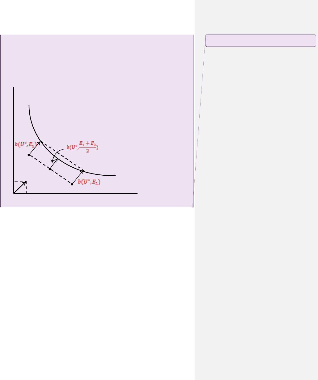
c. In the graph below, the benefit associated with any initial endowment is
the length of the vector from the initial endowment to the utility target
where the direction of the vector is given by the composition of the
elementary bundle.
d. In the graph below, two initial endowments are shown
12
( and )EE
. The
benefit for each endowment is also shown by the vectors in the graph. The
benefit is also shown for an initial endowment given by
12
( ) 2EE
. By
completing the parallelogram, it is clear that the convexity of the
indifference curve implies that
* * *
1 1 2 2
( , ) ( , 2) ( , ).b U E b U E E b U E
Hence the benefit function is concave in the initial endowments.
Commented [C4]: COMP: Please set all Greek letters in
italic.
x
y
y0
x0
E2
U*
E1
Commented [C5]: COMP: Please set X and Y in italic in
the figure.