
CHAPTER 17:
Capital and Time
The problems in this chapter are of two general types: (1) those that focus on
intertemporal maximization and (2) those that ask students to make fairly simple present
discounted value calculations. Before undertaking any of these, students should be sure to read
the Appendix in Chapter 17. The appendix is especially important for problems involving
continuous compounding because students may not have encountered that concept in earlier
courses.
Comments on Problems
concerns intertemporal allocation with initial endowments in both periods.
17.2 This is a present discounted value problem. I have found that the problem is most easily
solved using continuous compounding (see below), but the discrete approach is also
compounding.
17.4 This is a traditional capital theory problem involving trees. Students seem to have
difficulty in seeing their way through this problem and in interpreting the results. Hence,
instructors may wish to allow some time for discussion of it.
17.5 This problem is a discussion question that asks students to explore the logic of the U.S.
effective example of the time value of money.
17.6 This problem presents a discounted value example of life insurance sales tactics. Students
17.7 This problem is a simple numerical example of the “Hotelling rule” for natural resource
pricing developed in the text.

17.8 Capital gains taxation. This is a graphic problem that shows how changes in the interest
rate induce capital gains that might be taxed.

17.9 Precautionary saving and prudence. This is a simple example showing how uncertainty
can be incorporated into the saving model presented in the chapter. It shows that the third
derivative of the utility function matters.
shows, with a finite resource, monopoly pricing options are severely constrained.
17.11 Renewable timber economics. This is a continuation of Problem 17.4, which shows that
optimal timber harvesting rules may be a bit different once the possibility of replanting is
material in the chapter with a more explicit focus on the expected rate of return. It
describes the Sharpe ratio and uses the bound on that ratio to provide a simple example of
the equity premium puzzle.
17.13 Hyperbolic discounting. This behavioral problem introduces Laibson’s hyperbolic
utility function and provides a relatively intuitive presentation of the intertemporal
behavior implied by this function.
Solutions
17.1
a. The Lagrangian expression for this maximization problem is
2
1 2 1
() c
= U c , c + W c 1 + r
L
The first-order conditions for a maximum are
11
22
0,
(1 ) 0,
(1 ) 0,
cc
cc
U
Ur
W c c r
L
L
L
Commented [CE1]: COMP: [GLOBAL] Please set Lagrangian
ℒ instead of the L in the equation.
Commented [CE2]: COMP: [GLOBAL] Please set Lagrangian
ℒ instead of the L in the equation.

()
rt
e f t
17.5 a. Not at all, because there are no pure economic profits in the long run.
b. In long-run equilibrium: v = PK(r + d). Government taxes opportunity cost of
35
0.1
0
400 3879
t
dt = .
e
The salesman is wrong. The term policy represents a better value to this
consumer.
Analytical Problems
17.8 Capital gains taxation
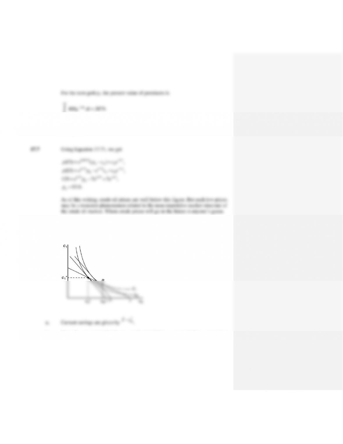
b. Once the one-period bonds are purchased, fall in r causes budget constraint to
rotate to Iʹ. Increase in utility from U0 to U1 (point B) represents a capital gain.
c. Accrued capital gains are measured by the total increase in ability to consume c0
(this is the “Haig–Simmons” definition of income) measured by distance IIʹ.

d. Realized capital gains are given by distance
*
0,B
cc
that is the present value of one-
period bonds that must be sold to attain the new utility-maximizing choice of cB.
e. The “true” capital gain is given by the value, in terms of c0, of the utility gain.
That is measured by II″. Notice that this is smaller than either of the “gains”
calculated in parts (c) or (d). Hence, the current practice of taxing realized gains,
while more appropriate than full taxation of all accrued gains, still amounts to
some degree of overtaxation because it neglects the effects on c1 consumption
opportunities.
17.9 Precautionary saving and prudence
a. In the context of uncertainty, the person will aim to maximize the total expected
utility. Thus, if consumption is certain in the current period and uncertain in the
next period, utility maximization will be achieved when the current marginal
utility from consumption is equal the expected marginal utility of consumption in
the next period, that is,
)()( 10 cUEcU
.
b. If
U
is convex, Jensen’s inequality gives
1 1)
[ ( )] ‘[ ( ].E U c U E c
So, we know that
).(‘)(‘ 11 p
cUcUE
Using the fact that utility maximization
)(‘)(‘ 10 cUEcU
).(‘)(‘ 10 p
cUcU
U
U
consistent with observed consumption growth, in part explaining the low real rate.
17.10 Monopoly and natural resource prices
U

a. If the resource is owned by a single firm, then the firm sets the market price.
Thus, the price in Equation 17.63 would be a function of q.
b. The Hamiltonian would be
1/
1/
1( ) ( ) ( ) ( ) ( ) ( ) .
rt b
b
d
H e q t q t c t q t q t x t
a dt
Differentiation with respect to t yields
0))()(())()(( rtrt etctRMetctMRr
. Diving by
rt
e
and using the
)11()11( bpRMbpMR
as in Equation 17.69.
17.11 Renewable timber economics
a. Since
2… for 1
1
xx x x
x
( ( ) ) ( )
11
rt
rt rt
f t w e f t w
V = w + w
ee
.
b.
2
( 1) ( ) [ ( ) ] 0
( 1)
rt rt
rt
dV e f t f t w re
dt e

So, for a maximum,
*
*
*
* * *
[ ( ) ]
( ) ( ) ( )
rt
rt
f t w re
f t rf t rV t
c. The condition implies that, at optimal
*
t
, the increased wood obtainable from
lengthening t must be balanced by: (1) the delay in getting the first rotation’s yield
and (2) the opportunity cost of a one-period delay in all future rotations’ yield.
d.
()ft
is asymptotic to 50 as
t
.
e.
*100.t
This is not “maximum yield” since tree continues growing after 100
years.
f. Now
*104.1.t
A lower interest rate lengthens the growing period.
17.12 More on the rate of return on a risky asset
a. Equation 17.37 is
()
( ) ( ) ( ) Cov( , ) Cov( , )
i
i i i i i
f
Ex
p E m x E m E x m x m x
R
.
Multiplication by
fi
Rp
and rearranging terms yields
( ) Cov( , ) Cov( , ),
f
i f i f i
i
R
E R R m x R m R
p
p

returns is about 0.16. So
(0.09 0.01) 0.16 0.5
. With
ln 0.01
c
this implies a
value for
of about 50—far above the value generally believed to characterize
17.13 Hyperbolic discounting
a. For the given utility function, the discount factors have the following values:
2
1, , ,
.
For
6.0
and
99.0
, the set of discount factor values are
2
1,0.594,0.594(0.99),0.594(0.99)
other words, long-term plans made in the current period are likely to be changed
in the next period, leading to a shortsighted behavior.
c. In period t, the MRS between ct+1 and ct+2 will be
).(/)( 21 tt cUcU
).(/)( 21 tt cUcU