
CHAPTER 16:
Labor Markets
Because the subject of labor demand was extensively treated in Chapter 11, the problems in this
chapter focus primarily on labor supply and on equilibrium in the labor market. Most of the labor
supply problems (16.1–16.3) start with the specification of a utility function and then ask
students to explore the labor supply behavior implied by the function. The primary focus of most
of the problems that concern labor market equilibrium is on monopsony and the marginal
expense concept (problems 16.5–16.7). Analytical problems are concerned with generalizing the
labor supply problems to consider risk, family labor supply, and intertemporal labor supply.
Comments on Problems
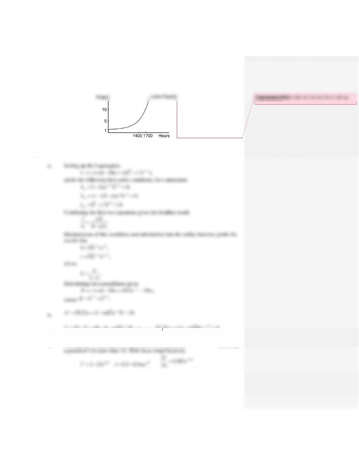
16.1 This problem is an algebraic example of labor supply that is based on a CobbDouglas
(=3/4 of 8,000) of leisure.
16.2 This problem uses the expenditure function approach to study labor supply. It shows why
income and substitution effects are precisely off-setting in the Cobb–Douglas case.
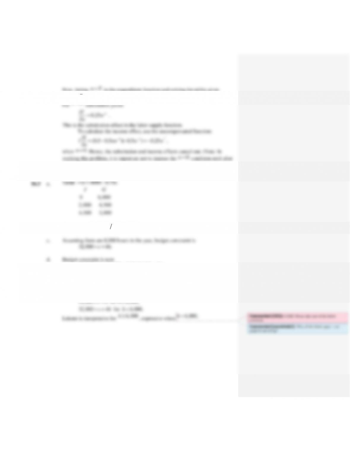
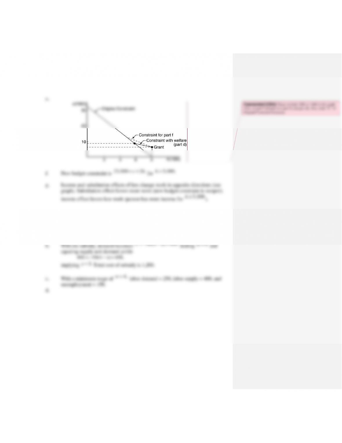
16.3 This problem is an application of labor supply theory to the case of means-tested income
transfer programs. The problem results in a kinked budget constraint. Reducing the
implicit tax rate on earnings (parts (f) and (g)) has an ambiguous effect on H since
equilibrium outcomes.
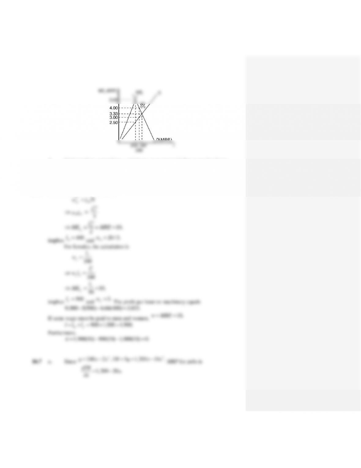
16.5 This problem is an illustration of marginal expense calculation. The problem also shows
that imposition of a minimum wage may actually raise employment in the monopsony
case.
16.6 This problem is an example of monopsonistic discrimination in hiring. The problem

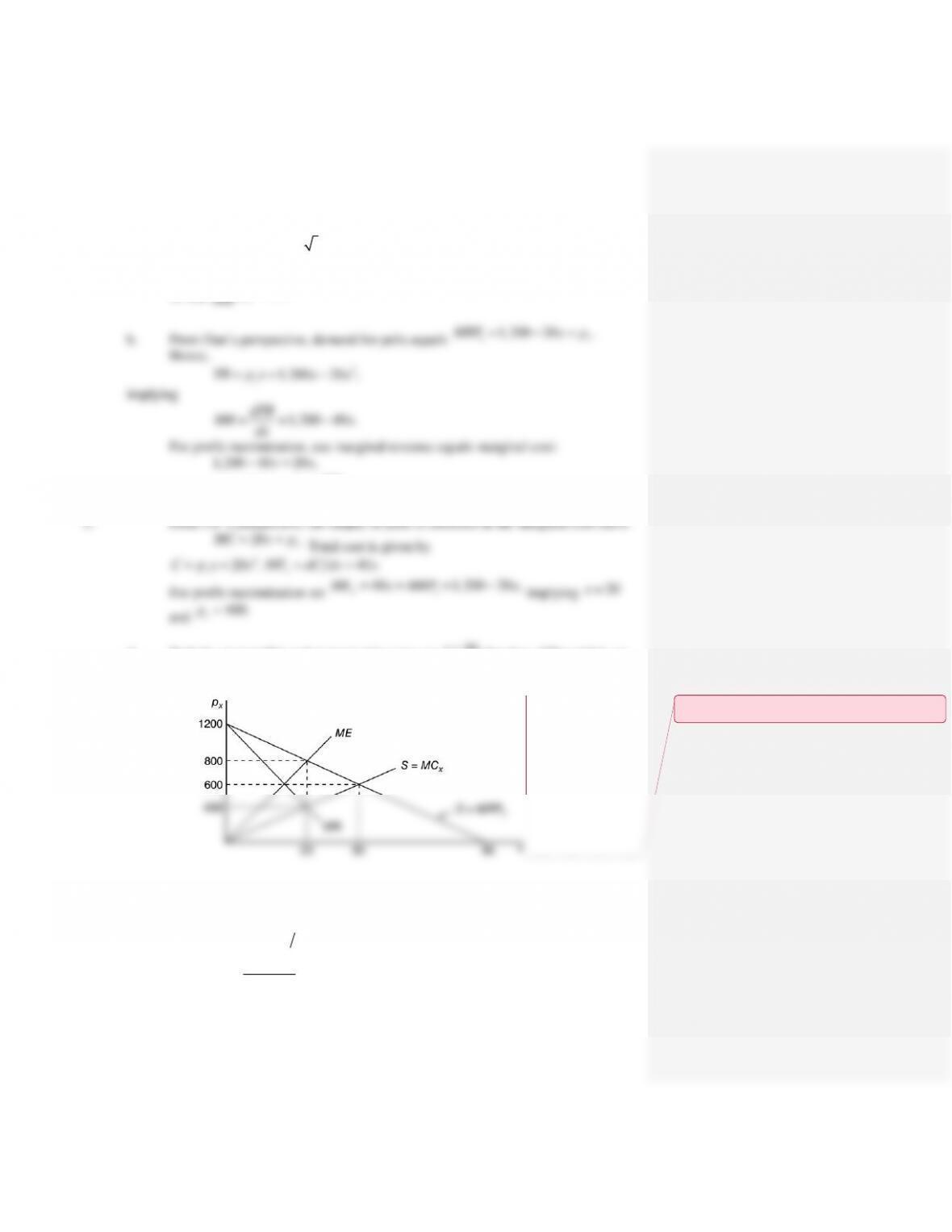
16.7 This is a bilateral monopoly problem for an input (here, pelts). Students may get confused
on what is required here, so they should be encouraged first to take an a priori graphical
approach and then try to add numbers to their graph. In that way, they can identify the
relevant intersections that require numerical solutions.

16.8 This problem is a numerical example of the union–employer game illustrated in Example
16.5.
Analytical Problems
16.9 Compensating wage differentials for risk. This problem develops the idea of a
production.” The functional forms specified here are so general that this problem should
be regarded primarily as a descriptive one that provides students with a general
framework for discussing various possibilities.
16.11 A few results from demand theory. This problem shows how many problems in labor
supply theory can be addressed using demand theory concepts from Part 2 of the text.
16.12 Intertemporal labor supply. This problem is an introduction to some general concepts
in the theory of multiperiod labor supply. Because time has not yet been explicitly
introduced, however, the results pertain only to a situation with no discounting.
Solutions
16.1 a. With 8,000 hours/year, full income is $40,000. If 75 percent of this is
devoted to eisure, this $30,000 will “buy” 6,000 hours of leisure at $5 per hour. Hence,
work time will be 2000 hours.
b. Full income is now $44,000, so this person will devote $33,000 to leisure. This
16.2
c.
24 48 (1 ) .
cc
l h Uw K
Clearly,
1
(1 ) 0
c
l w UKw
.
d. The algebra is considerably simplified here by assuming
0.5, 2K
and using
Commented [CE1]: COMP: Set 1400 and 1700 as 1,400 and
1,700, respectively.
Now, letting
nE
in the expenditure function and solving for utility gives
0.5 0.5
0.5 0.5 .U w nw
0,n
taking all derivatives.)
b.
0G
when
6,000 0.75 8,000.I
32,000 38,000 0.75(32,000 4 )
14,000 3
4
Gh
h
ch
for
6,000.h
Hence, the budget constraint is kinked at
6,000.h
Its
mathematical form is
14,000 for 6,000,
32,000 4 for 6,000.
c h h
c h h
Leisure is inexpensive for
6,000h
, expensive when
6,000.h
Commented [CE2]: COMP: Please take care of the below
comment.
Commented [wenichols3]: Why all this blank space – can
graph be moved up?
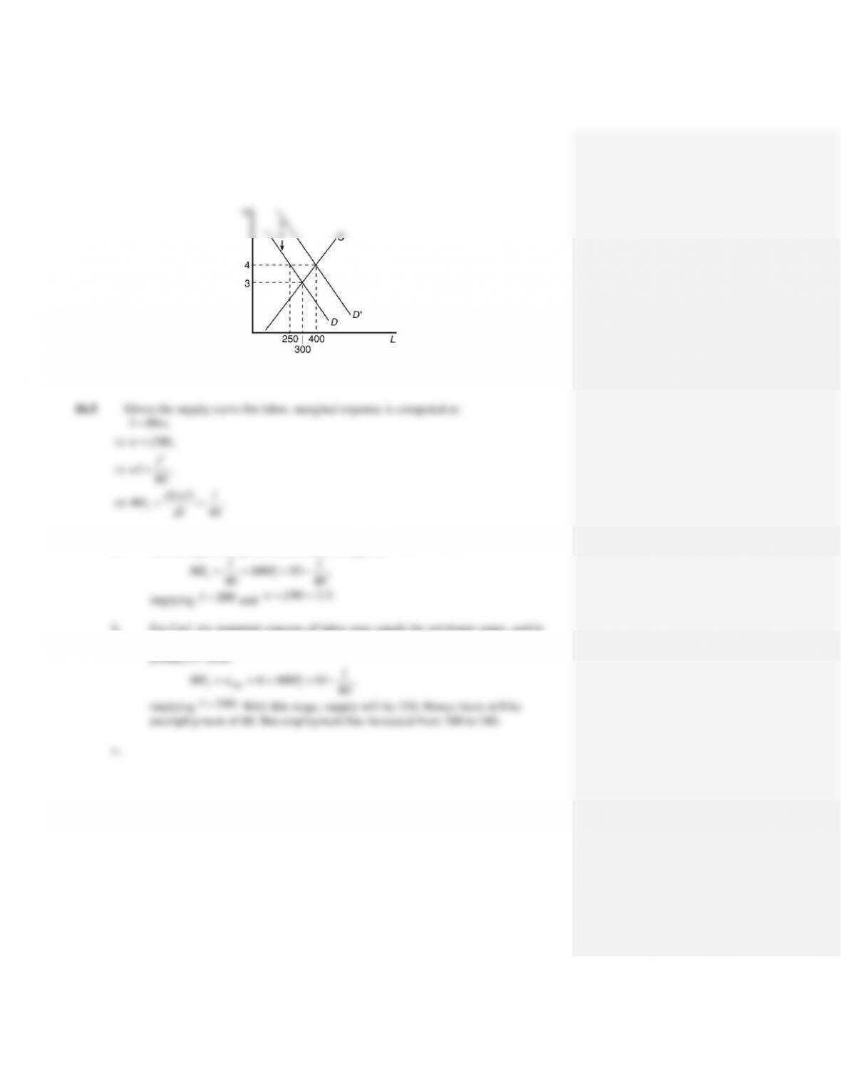
16.4 Labor demand is
50 450,Lw
and labor supply is
100 .Lw
a. Setting labor demand equal to supply yields
3,w
300.L
50( ) 450.L w s
a. For monopsonist, profit maximization required
ll
ME MRP
:
10 ,
ll
ll
ME MRP
equilibrium the marginal expense of labor will equal the marginal revenue
workers employed. Under monopsony, a minimum wage may result in higher
wages and more workers employed.
16.6 First, look at the case of males:
2
3/2
0.5
9
3
10,
m
m
m
m
mm
m
ll
wl
l
wl
l
ME = = MRP
8 6.25
9
11
implying
1 2.75 ,
or
1 2.75 0.36.
Analytical Problems
16.9 Compensating wage differentials for risk
Considering the first (riskless) job,
2
( ) 100 0.5U y y y
and
y wl
with
5w
and
8l
implies
(40) 3,200.U
That is,
a.
12
hw
and
21
hw
are both probably positive because of the income effect.
b.
11
( ),c f h
so, optimal choice would be to choose
1
h
so that
1.fw
This would
probably lead person 1 to work less in the market. That may in turn lead person 2
to choose a lower level of
2
h
on the assumption that
1
h
and
2
h
are substitutes in
1
1
11
( , ) 1
( ) 1
(1 ) ( ) .
V w n n
wn
n w w
n w w n
Dividing the first equation by the second yields (after some manipulation)
(1 ) .
n
lw
This is the labor supply function given in Equation 16.24.
b. Using the logic of the development of the Slutsky equation, for any consumption
good
.
i i i
U
x x x
h
w w I
Hence, for any normal good, the income effect in this expression will be positive.
This positive effect will be reinforced for goods that are Hicksian complements
with labor (substitutes for leisure). The substitution effect will be negative,
however, for goods that are Hicksian substitutes for labor (complementary with

Notice that since
,lw
e
is likely to be positive,
.
l
ME w
If
,,
lw
e
then
.
l
ME w
16.12 Intertemporal labor supply
1
1
1.
h
c
U
MRS w
U
An increase in initial wealth should increase both leisure and consumption
assuming they are normal goods.
b. The equation just says that second-period indirect utility is a function of the
expression to interpret derivatives. The indirect utility function arises from the
problem
max [ ( , )]E U c h

d. A certain increase in second-period wages is similar to an increase in initial
wealth. The first-period effects therefore should be to increase both consumption
and leisure. The effects on second-period labor supply are uncertain because