
CHAPTER 14:
Monopoly
The problems in this chapter deal primarily with marginal revenue-marginal cost calculations in
different contexts. For such problems, students’ primary difficulty is to remember that the
marginal revenue concept requires differentiation with respect to quantity. Often students choose
to differentiate total revenue with respect to price and then get very confused on how to set this
equal to marginal cost. Of course, it is possible to phrase the monopolist’s problem as one of
choosing a profit-maximizing price, but then the inverse demand function must be used to derive
a marginal cost expression.
The analytical and behavioral problems in this chapter introduce students to some state-
of–the-art research on monopoly reflected in recent academic articles.
Comments on Problems
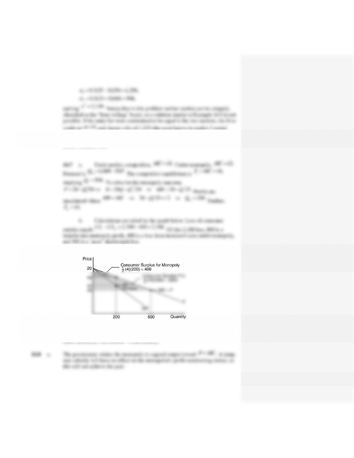
14.1 This problem is a simple marginal revenue-marginal cost and consumer surplus
computation.
14.2 This problem is an example of the MR = MC calculation with three different types of cost
curves.
14.3 This problem is an example of the MR = MC calculation with three different demand and
marginal revenue curves. The problem also illustrates the “inverse elasticity” rule.
14.4 This problem examines graphically the various possible ways in which shift in demand
may affect the market equilibrium in a monopoly.
14.5 This problem introduces advertising expenditures as a choice variable for a monopoly.
The problem also asks the student to view market price as the decision variable for the
monopoly.
14.6 Note: This problem has been subtly revised from the previous edition; the numbers for
production and transportation cost are now different, helping students see where each
distinctly shows up in the calculations. This is a price-discrimination example in which
markets are separated by transport costs, showing how the price differential is
constrained by the extent of those costs. Part (d) asks students to consider a simple two-
part tariff.
14.7 This problem shows how the welfare cost of monopoly may be larger than in the
traditional case if the monopoly has higher costs.
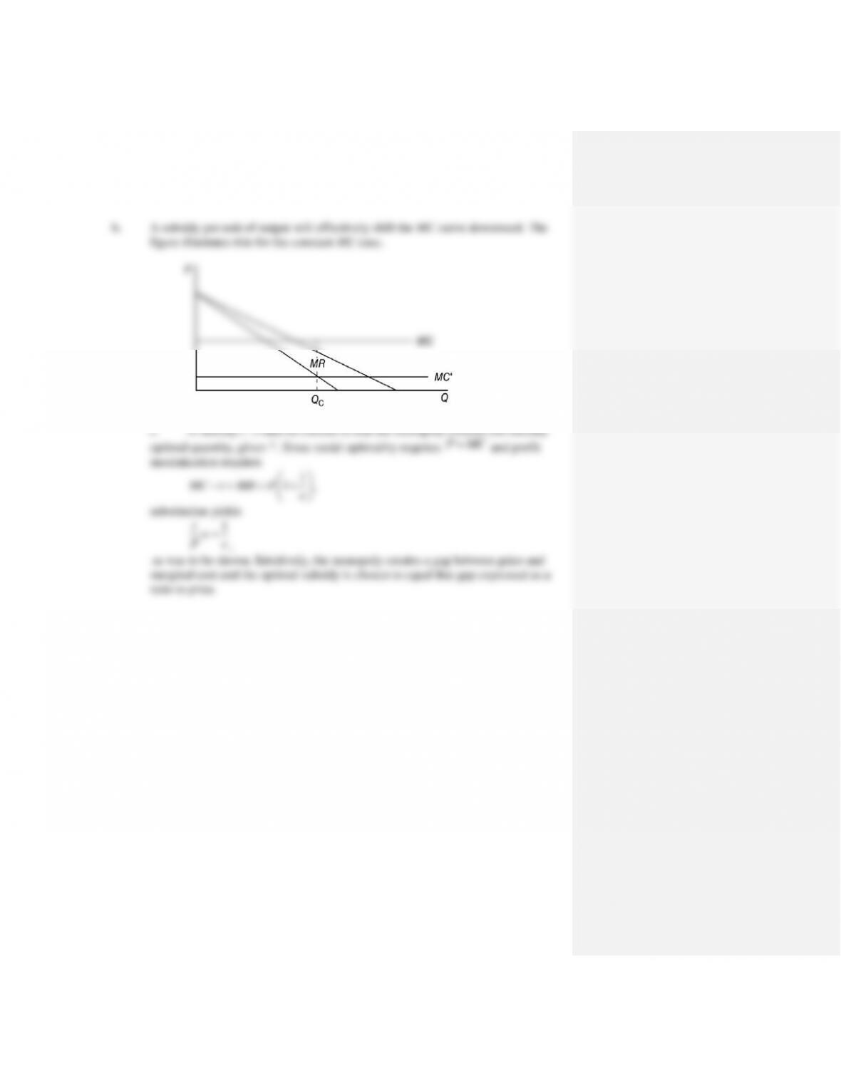
14.8 This problem examines some issues in the design of subsidies for a monopoly.
14.9 This problem involves quality choice. The result shows that, in this case, the monopoly
and competitive choices are the same (though output levels differ).
Analytical Problems
14.11 Flexible functional forms. This problem has students run through the standard
monopoly analysis but for a class of flexible functional forms introduced in a recent
influential paper by Fabinger and Weyl (2015). While slightly complicated, the
functional forms allow for U-shaped average cost curves and realistic demand shapes.
Behavioral Problem
14.13 Shrouded prices. This problem introduces students to the problem of shrouded prices, a
505–540. More on whether competition uncovers shrouding to come in the next chapter.
Solutions
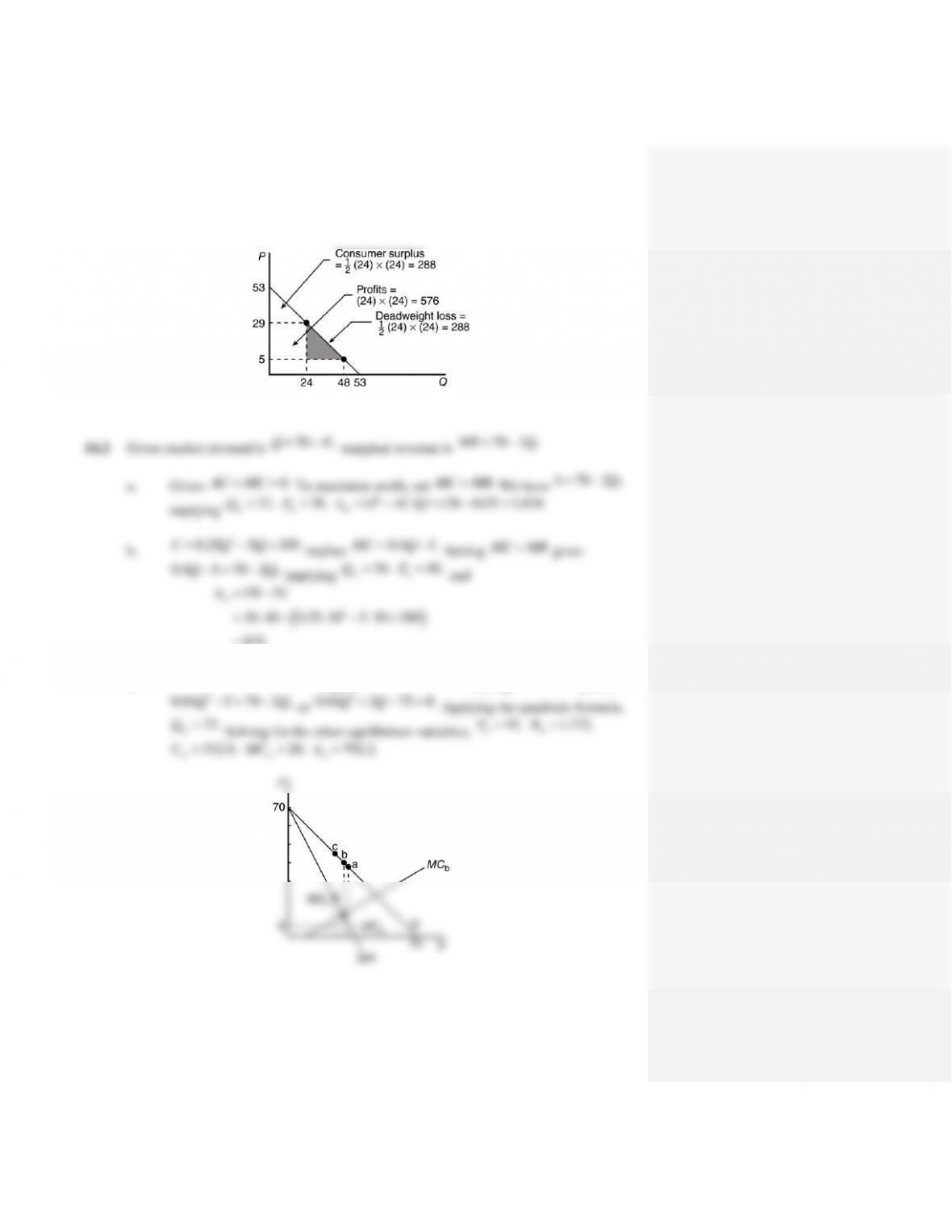
14.1 a. Given
53 .PQ
Then
2
53 ,TR PQ Q Q
implying
53 2 .MR Q
Profit
maximization yields
53 2 5,MR q MC
implying
24,
m
Q
29,
m
P
and
576.
mP AC Q
2
30 40 0.25 30 5 30 300
825.
mTR TC
c.
3
0.0133 5 250C Q Q
implies
2
0.04 5.MC Q
Setting
MR MC
yields
2
0.04 5 70 2 ,QQ
or
2
0.04 2 75 0.QQ
Applying the quadratic formula,
25.
m
Q
Solving for the other equilibrium variables,
45,
m
P
1,125,
m
R
332.8,
m
C
20,
m
MC
792.2.
m
60 ,QP
60 2 .MR Q
b. Given
10AC MC
and
100 2 ,QP
implying
90 4 .MR Q
For profit
10 90 4 20.
MC MR Q Q
equilibrium variables,
30
m
P
and
40 30 40 10 800.
m
π = (40)(30) –
(40)(10) = 800.
Note: Here the inverse elasticity rule is clearly illustrated:
Problem part
,QP
QP
e =
PQ
1
Q,P
P MC
= P
e
(a)
1 35 25 1.4
0.71 35 10 35
(b)
0.5 50 20 1.25
0.80 50 10 50
(c)
2 30 40 1.5
0.67 30 10 30
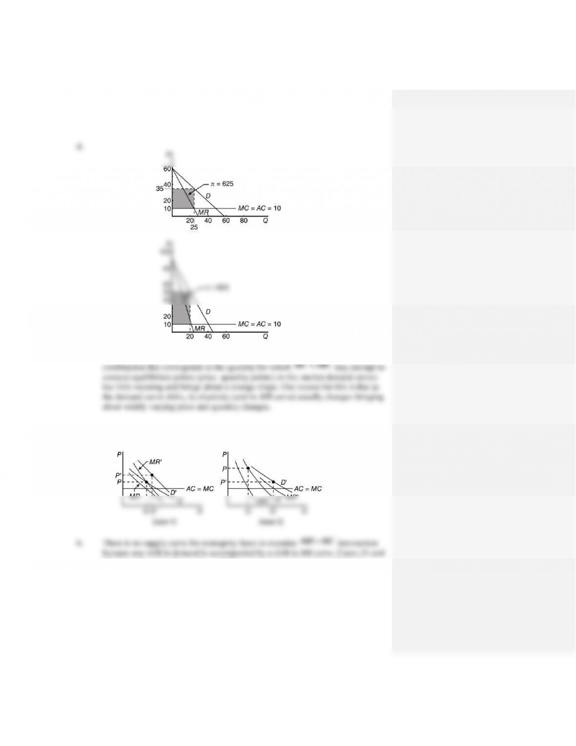
The supply curve for a monopoly is a single point, namely, that quantity–price
14.4 a.
(2) above show that P may rise or fall in response to an increase in demand.
c. Can examine this using inverse elasticity rule:
PP
e = = .
14.5 Given
2
20 1 0.1 0.01 .Q P A A
Let
2
1 0.1 0.01 .K A A
Then
0.1 0.02dK dA A
and
2
20 200 10 15 .
PQ C
P P K P K A
1.5 0.5 0,
d = A=
implying
3,A
5(1 0.3 0.09) 6.05,
m
Q
90.75,
m
R
60.5 15 3 78.5,
m
C
and
12.25;
m
this represents an increase over the
case
0.A
across both markets are
(30 5) 25 (20 5) 30 1,075.
b. If the producer ignores the problem of arbitrage among consumers, the price
and
*1,008.33.
( ) ,
i
T Q = + mQ
1
0.5(55 5)(50) 1,250,
0.5(35 5)(60) 900,
could set
0m
and charge a fee of 1,225 (the most buyers in market 2 would
pay). This would yield profits of
2,450 125 5 1,825,
which is inferior to
profits obtained with
( ).
i
TQ
c.
The new feature of the analysis is that costs are not given, but vary
with the market structure, rising under monopoly. The possibility of higher costs
under monopoly was dubbed “X–inefficiency.”
c. A subsidy (