
CHAPTER 13:
General Equilibrium and Welfare
WelfareExternalities and Public Goods
The problems in this chapter focus primarily on the simple two-good general equilibrium model
in which “supply” is represented by the production possibility frontier and “demand” by a set of
indifference curves. One shortcoming of this approach is that students do not see the interaction
between output and input markets. Problems 13.7 and 13.8 seek to remedy this by using the
computer general equilibrium model presented in the chapter. The Analytical Problems in the
chapter illustrate a few general equilibrium “theorems,” but no very formal proofs are intended.
Comments on Problems
13.1 This problem repeats an example from Chapter 1 in which the production possibility
frontier is concave (a quarter ellipse). It is a good starting problem because it involves
very simple computations.
13.2 This problem is a simple example of general equilibrium with linear production functions
and differing preferences among the two people in the economy.
13.3 This problem is a fixed-proportions example that yields a concave production possibility
frontier. This is a good initial problem although students should be warned that calculus-
type efficiency conditions do not hold precisely for this type of problem.
13.4 This problem uses a quarter-circle production possibility frontier and a Cobb–Douglas
utility function to derive an efficient allocation. The problem then proceeds to illustrate
the gains from trade. It provides a good illustration of the sources of those gains.
13.5 This problem provides a numerical example of an Edgeworth Box in which efficient
allocations are easy to compute because one individual wishes to consume the goods in
fixed proportions.
13.6 This provides an example of efficiency in the regional allocation of resources. The
problem could provide a good starting introduction to mathematical representations of
comparative versus absolute advantage or for a discussion of migration. To make the
problem a bit easier, students might be explicitly shown that the production possibility

frontier has a particularly simple form for both the regions here (e.g., for region A it is
22
100xy
).
13.7 This problem uses the computer model to examine the consequences of various changes
in preferences or technology. Having students try to explain why things turn out the way
they do is a good way to build intuition.
Analytical Problems
13.8 Tax equivalence theorem. This problem uses the computer simulation model to shows
the formal equivalence between input and output taxes.
13.11 An example of Walras’ law. This problem is a algebraic example of how Walras’ law
can be used to find the excess demand function for good 1.
13.12 Productive efficiency with calculus. This problem illustrates how the simple two-good
13.13 Initial endowments, equilibrium prices, and the first theorem of welfare economics.
13.14 Social welfare functions and income taxation. This problem explores the complex
relationship between social welfare and the appropriate tax function.
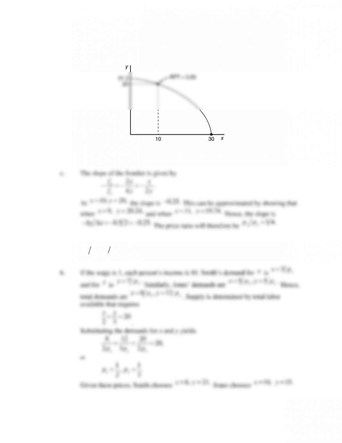
13.1 a. The frontier is a quarter ellipse.
b.
2
9 900,x
so,
10x
and
20.y
13.2 a.
32
xy
pp
.
16, 36xy
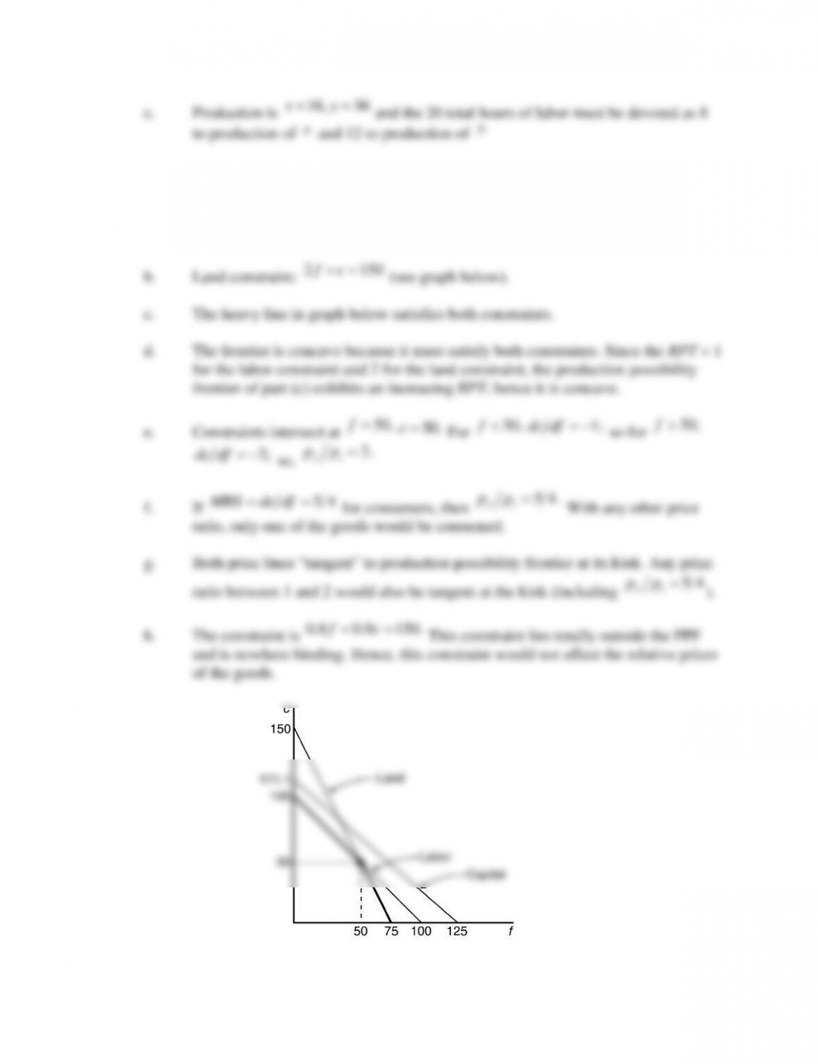
13.3 Let f denotes food and c cloth.
a. Labor constraint:
100fc
(see graph below).
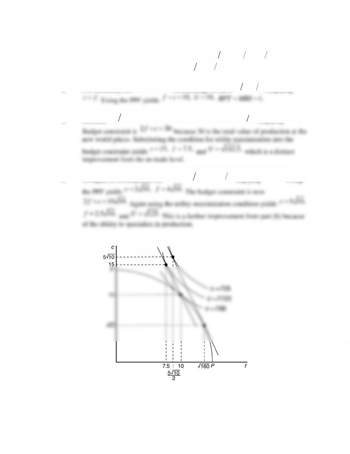
13.4 The PPF has the form
22
200.fc
2 2 .RPT dc df f c f c
Consumer preferences imply
.
fc
MRS U U c f
a. For efficiency, set
.MRS RPT
Substituting, we have
f c c f
, implying
.cf
Using the PPF yields
10,fc
10,U
1.RPT MRS
b. Demand:
2.
fc
pp
For utility maximization,
2,MRS c f
implying
2.cf
2 30fc
c. To adjust to world prices, set
2,
fc
RPT p p f c
implying
2.fc
Using
2 10,c
4 10.f
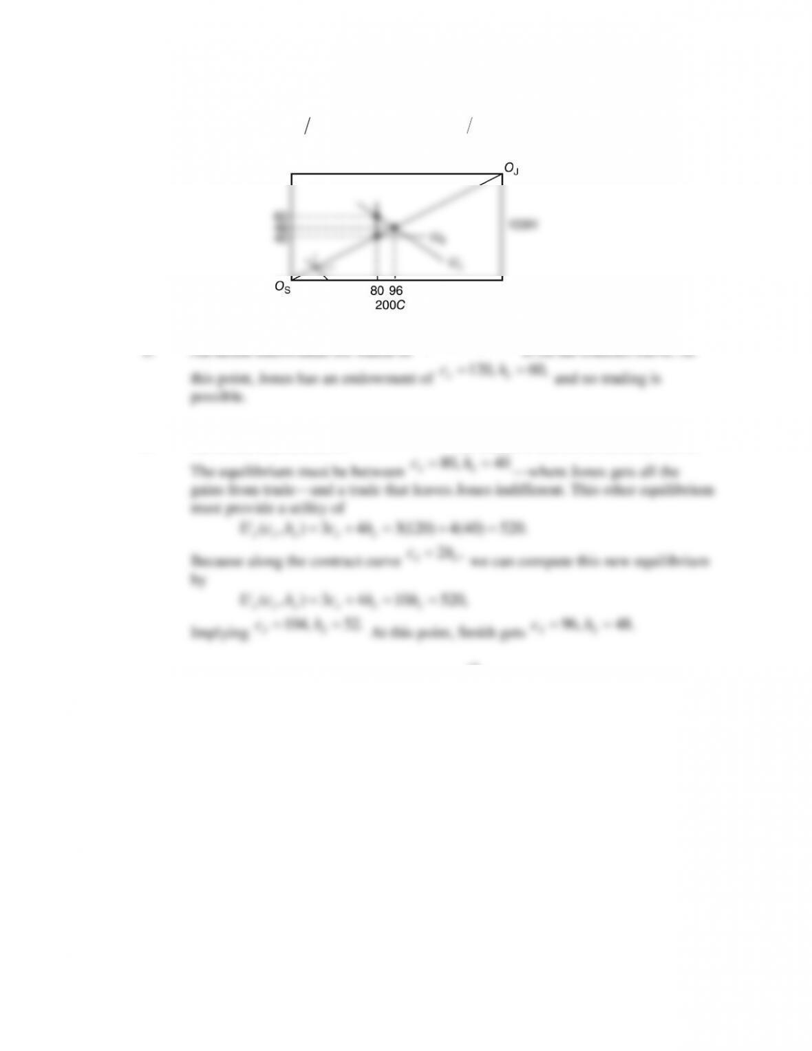
13.5 a. Contract curve is straight line with slope of 0.5. The only price
ratio in equilibrium is
(for Jones) 3 4.
ch
p p MRS
b. An initial endowment for Smith of
80, 40
SS
ch
is on the contract curve. At
120, 60,
JJ
ch
c. An initial endowment of
80, 60
SS
ch
for Smith is not on the contract curve.
80, 40
SS
ch