therefore reduce the number of firms.
Analytical Problems
12.10. Ad valorem taxes
[ (1 )] 0,
( ) 0,
(1 ) 0 ,
0.
P P P p
P
D P t Q
S P Q
dP dQ dP dQ
D P D t D D P
dt dt dt dt
dP dQ
Sdt dt
Writing this in matrix notation:
1
10
PP
P
DDP
dP dt
S dq dt
and applying Cramer’s rule:
* * * ,
,,
1
01 1 ln
or .
1
1
P
DP
PP
PP P P P S P D P
P
DP
e
D P D
dP dP d P
D
dt S D P dt dt S D e e
S
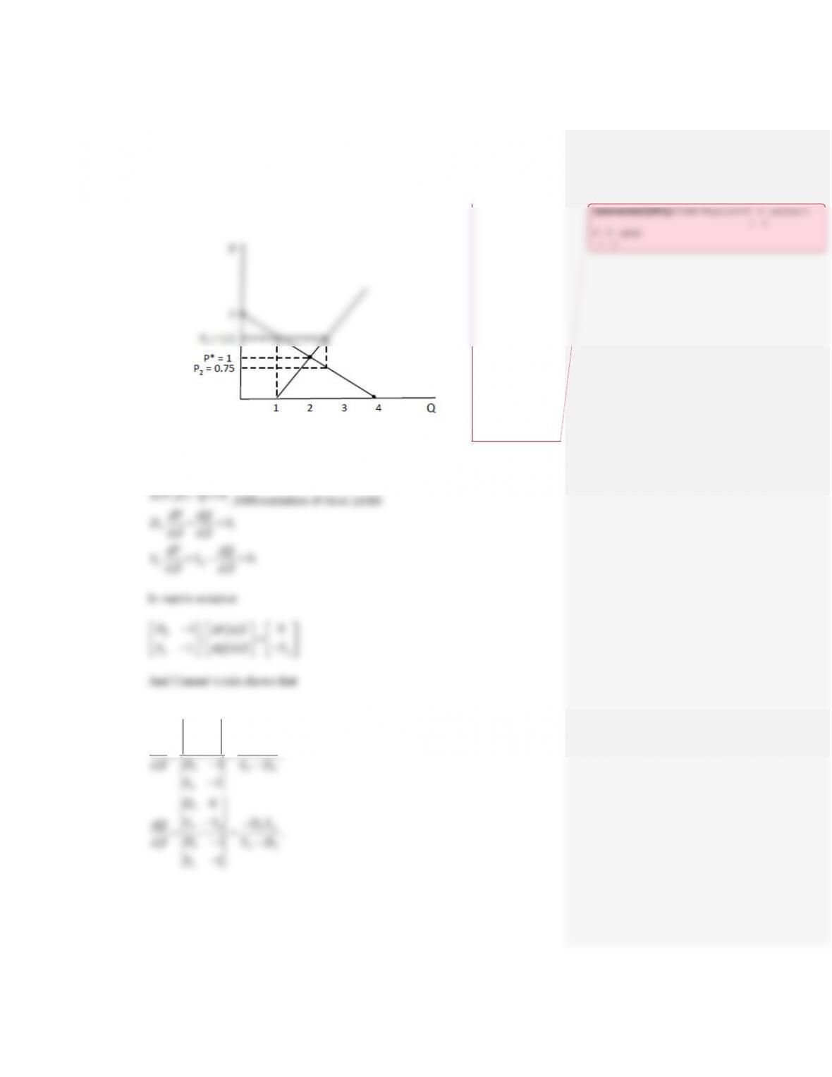
P
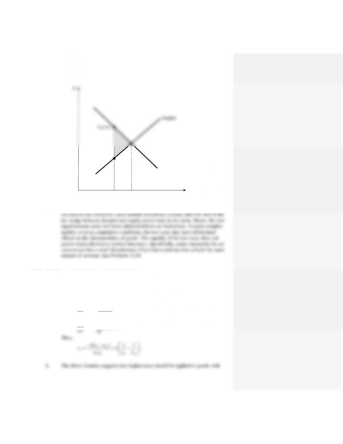
Q
Supply
Demand
PS (1+t)
PS
QSQ0
c. Under perfect competition the tax “wedge” diagram shows that if a unit tax and an
12.11 The Ramsey formula for optimal taxation
a. Use the deadweight loss formula from Problem 12.9:
11
( ) .
0.5 2 0.
0.
nn
i i i i
ii
DS i i i i i
i S D
n
i i i
L DW t T t p x
ee
Lt p x p x
t e e
LT t p x
market separately), ignoring the general equilibrium interactions between
markets. Also, income effects and cross-price elasticities are not taken into
account.
12.13 More on the comparative statics of supply and demand
a. Shifts in supply: Assume demand is given by
( ) 0D P Q
and supply by
( , ) 0S P Q
. Differentiation of these yields
0,
0.
P
P
dP dQ
Ddd
dP dQ
SS
dd
In matrix notation
0
1
1
P
P
DdP d
S
S dQ d
And Cramer’s rule shows that
01
1,
1
1
0
.
1
1
PPP
P
P
PP
PPP
P
SS
dP
D
d S D
S
D
SS DS
dQ
D
d S D
S
Commented [CE1]: COMP: Please set P, P
1
, P
2
, and Q as P,
P
1
, P
2
, and Q.
Hence, if
**
0, then 0 and 0.S dP d dQ d
This is precisely the lesson
from introductory economics—a shift outward in the supply curve lowers price
i. The analysis in the chapter shows that
*
*P
dQ d S
dP d
. With sufficient
observations on the impact of differing values of
, one could identify the slope
of the supply curve.
ii. Part (a) of this problem shows that
*
*P
dQ d D
dP d
. With sufficient observations
on the impact of differing values of
, one could identify the slope of the
demand curve.
iii. If the same parameter shifts both curves it is not possible to identify the
slope of either of them.
12.14 The Le Chatelier Principle
a. Here are Equations 12.24:
* * * *
**
0 or
0.
PP
P
dP dQ dP dQ
D D D D
d d d d
dP dQ
Sdd
Differentiation with respect to t yields
22
22
0,
0.
P
P Pt
d P d Q
Dd dt d dt
d P dP d Q
SS
d dt d d dt
b. Cramer’s rule can now be used to solve for the second-order partials:
2
01
1.
1
1
Pt Pt
PPP
P
dP dP
SS
dP dd
D
d dt S D
S
This expression shows that
2 and
d P dP
d dt d
are of opposite signs. That is, the
effect of an outward demand shift on increasing price diminishes over time.
Similarly, a reduction in demand initially reduces price, but then price rises over
time back toward the old equilibrium. The Le Chatelier principle therefore
captures the way in which entry and exit affect price in the model of competitive
pricing developed in this chapter.
c. Again, we use Cramer’s rule:
2
0
,
P
P Pt
P Pt P Pt P
P P P P P P
D
DS dQ
dP dP
SS DS Sd
dQ dd
d dt S D S D S D
where the final equation uses the combined results of Equations 12.26 and 12.27.
Because
0 and S 0
P Pt
D
, this result shows that the effect of
on equilibrium
d. See answers to parts (b) and (c) above.