
The problems in this chapter focus mainly on the relationship between production and cost
functions. Most of the examples developed are based on the Cobb–Douglas function (or its CES
generalization), although a few of the easier ones employ a fixed proportions assumption. Two of
the problems (10.7 and 10.8) make use of Shephard’s lemma since it is in describing the
relationship between cost functions and (contingent) input demand that this envelope-type result
is most often encountered. The analytical problems in this chapter focus on various elasticity
concepts, including the introduction of the Allen elasticity measures.
Comments on Problems
10.1 An introduction to the concept of “economies of scope.” This problem illustrates the
connection between that concept and the notion of increasing returns to scale.
10.2 A simplified numerical Cobb–Douglas example in which one of the inputs is held fixed.
10.3 A fixed proportion example. The very easy algebra in this problem may help to solidify
basic concepts.
10.4 This problem derives cost concepts for the Cobb–Douglas production function with one
10.5 Another example based on the Cobb–Douglas with fixed capital. Shows that in order to
10.6 This problem focuses on the Cobb–Douglas cost function and shows, in a simple way,
how underlying production functions can be recovered from cost functions.
10.7 This problem shows how contingent input demand functions can be calculated in
10.8 Famous example of Viner’s draftsman. This may be used for historical interest or as a
CHAPTER 10:
Cost Functions
10.9 Generalizing the CES cost function. Shows that the simple CES functions used in the
chapter can easily be generalized using distributional weights.
10.10 Input demand elasticities. Develops some simple input demand elasticity concepts in
10.11 The elasticity of substitution and input demand elasticities. Ties together the concepts
10.12 The Allen elasticity of substitution. Introduces the Allen method of measuring
substitution among inputs (sometimes these are called Allen/Uzawa elasticities). Shows
that these do have some interesting properties for measurement, if not for theory.
Solutions
10.1 a. By definition, total costs are lower when both
1
q
and
2
q
are produced by
12
where
12
1 2 1
1
( , ) ( ,0),
C q q C q
qq
implying
1 1 2 1
( , ) ( ,0).
q C q q Cq
10.2 a. Substituting into the production function,
0.5 0.5 30 .
when
225J
when
450.q
b. Because Smith’s effort is sunk, to compute marginal cost we only need to
2
900
q
J
900
Thus,
24 2 .
900 75
C q q
MC
q
10.3 Given
min 5 ,10 .q k l
a. In the long run, no input should be wasted. Hence,
5 10 ,k l q
implying
2 5.k l q
Thus,
(2 )
C = vk wl
v l wl
qq
10 ,
10
.
10
STC v w
SAC = +
qq
STC w
SMC q
If
5,l
then
50. q =
It is impossible to produce more than 50 in the short
run. Hence,
STC SAC SMC
for
50.q
10
qq
c. Substituting
1v
and
3w
into the formulae from the previous parts, in the long
run,
1 2.AC = MC
In the short run, for
50,q
10 3 ,
10
STC
SAC = +
qq
10.4 Given
2,q = kl
100.k =
a. Since
2 100 ,q = l
20 .q = l
Rearranging,
,
20
q
l =
50
SC q
SMC = .
q
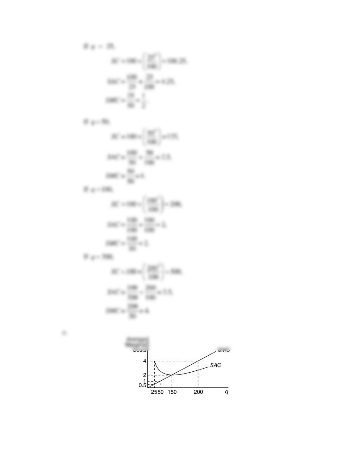
d. As long as the marginal cost of producing one more unit is below the average-cost
curve, average costs will be falling. Similarly, if the marginal cost of producing
one more unit is higher than the average cost, then average costs will be rising.
Therefore, the SMC curve must intersect the SAC curve at its lowest point.
e. Since
1
2,q = k l
2
1
= 4 ,kl
q
implying
2
1
= .
4
q
lk
Substituting,
2
11
1
4
wq
f. Deriving the first-order condition from the previous expression,
2
2
11
0.
4
SC wq
= v
kk
g. Substituting first for
l
and then for
1
k
into the cost function,
11
2
1
1
2
()
4
2
24
,
C = vk + wl k
q
= vk w k
q w wq v
v +
v q w
= q vw
(a special case of Example 10.2).
h. If
4 w
and
1,v
in the long run,
2 . Cq
1200k
1
( 200) 200 .
200
2
q
SC k = = +
This is tangent to the long-run cost function for
200,q
as one can verify
400 .SC C
Finally, fixing
1400k
in the short run,
1
( 400) 400 .
400
2
q
SC k = = +
This is tangent to the long-run cost function for
400,q
as one can verify
800 .SC C