
WHAT’S NEW IN THE EIGHTH EDITION:
There are no major changes to this chapter.
LEARNING OBJECTIVES:
By the end of this chapter, students should understand:
why policymakers face a short-run trade-o between ination and unemployment.
why the ination-unemployment trade-o disappears in the long run.
how supply shocks can shift the ination-unemployment trade-o.
the short-run cost of reducing ination.
589
© 2018 Cengage Learning®. May not be scanned, copied or duplicated, or posted to a publicly accessible website,
in whole or in part, except for use as permitted in a license distributed with a certain product or service or otherwise
on a password-protected website or school-approved learning management system for classroom use.
THE SHORT-RUN
TRADE-OFF BETWEEN
INFLATION AND
UNEMPLOYMENT
35

590 ❖ Chapter 35/The Short-Run Trade-o between Ination and Unemployment
how policymakers’ credibility might aect the cost of reducing ination.
CONTEXT AND PURPOSE:
Chapter 35 is the @nal chapter in a three-chapter sequence on the economy’s short-run
uctuations around its long-term trend. Chapter 33 introduced aggregate supply and
aggregate demand. Chapter 34 developed how monetary and @scal policies aect aggregate
demand. Both Chapters 33 and 34 addressed the relationship between the price level and
output. Chapter 35 will concentrate on a similar relationship between ination and
unemployment.
The purpose of Chapter 35 is to trace the history of economists’ thinking about the
relationship between ination and unemployment. Students will see why there is a
temporary trade-o between ination and unemployment, and why there is no permanent
trade-o. This result is an extension of the results produced by the model of aggregate
supply and aggregate demand where a change in the price level induced by a change in
aggregate demand temporarily alters output but has no permanent impact on output.
KEY POINTS:
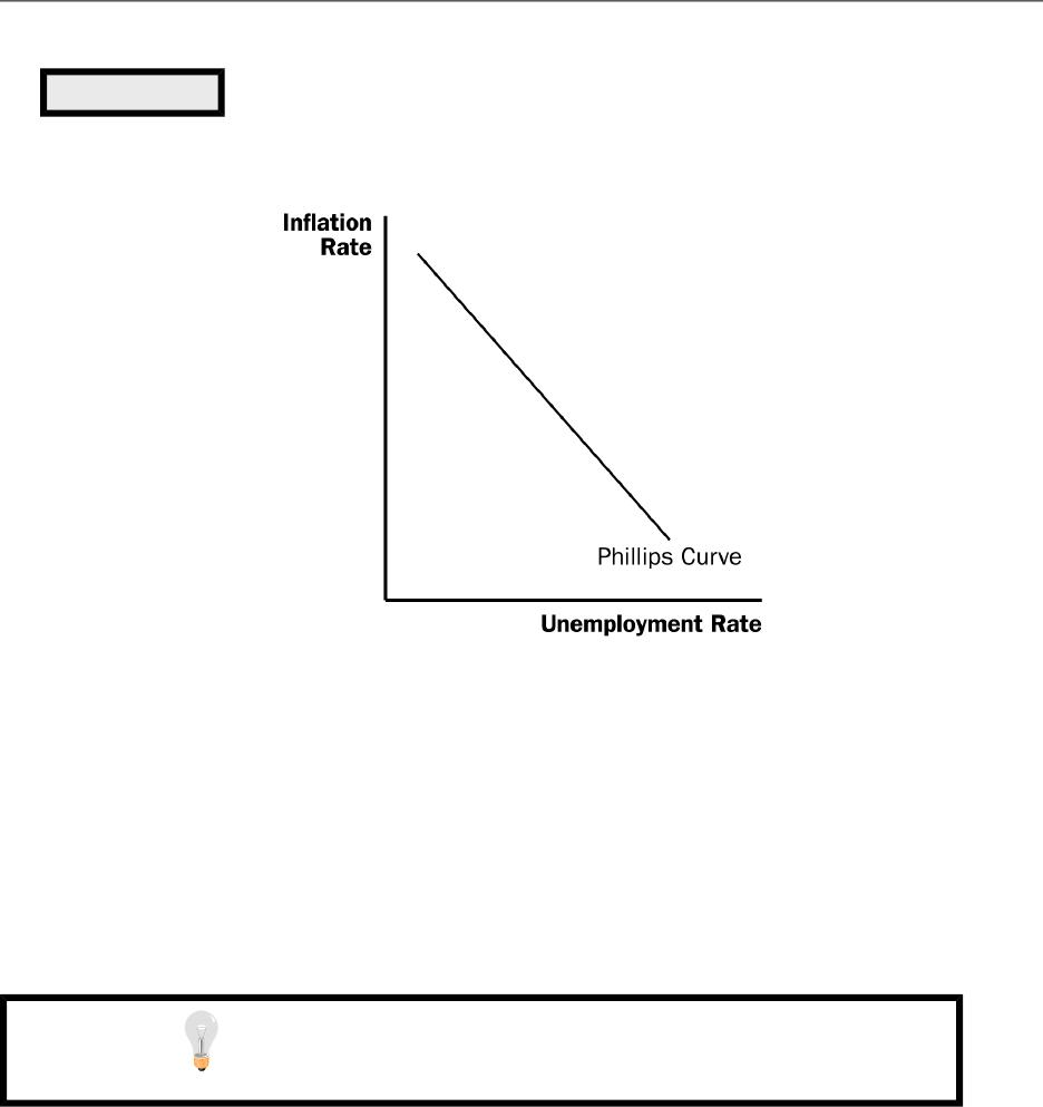
The Phillips curve describes a negative relationship between ination and
unemployment. By expanding aggregate demand, policymakers can choose a point on
the Phillips curve with higher ination and lower unemployment. By contracting
aggregate demand, policymakers can choose a point on the Phillips curve with lower
ination and higher unemployment.
The trade-o between ination and unemployment described by the Phillips curve holds
only in the short run. In the long run, expected ination adjusts to changes in actual
ination, and the short-run Phillips curve shifts. As a result, the long-run Phillips curve is
vertical at the natural rate of unemployment.
The short-run Phillips curve also shifts because of shocks to aggregate supply. An
adverse supply shock, such as an increase in world oil prices, gives policymakers a less
favorable trade-o between ination and unemployment. That is, after an adverse
© 2018 Cengage Learning®. May not be scanned, copied or duplicated, or posted to a publicly accessible website,
in whole or in part, except for use as permitted in a license distributed with a certain product or service or otherwise
on a password-protected website or school-approved learning management system for classroom use.

Chapter 35/The Short-Run Trade-o between Ination and Unemployment ❖ 591
supply shock, policymakers have to accept a higher rate of ination for any given rate of
unemployment, or a higher rate of unemployment for any given rate of ination.
When the Fed contracts growth in the money supply to reduce ination, it moves the
economy along the short-run Phillips curve, which results in temporarily high
unemployment. The cost of disination depends on how quickly expectations of ination
fall. Some economists argue that a credible commitment to low ination can reduce the
cost of disination by inducing a quick adjustment of expectations.
CHAPTER OUTLINE:
I. The Phillips Curve
A. Origins of the Phillips Curve
1. In 1958, economist A. W. Phillips published an article discussing the negative
correlation between ination rates and unemployment rates in the United
Kingdom.
2. American economists Paul Samuelson and Robert Solow showed a similar
relationship between ination and unemployment for the United States two years
later.
3. The belief was that low unemployment is related to high aggregate demand, and
high aggregate demand puts upward pressure on prices. Likewise, high
unemployment is related to low aggregate demand, and low aggregate demand
pulls price levels down.
4. De@nition of Phillips curve: a curve that shows the short-run trade-o.
between in0ation and unemployment.
© 2018 Cengage Learning®. May not be scanned, copied or duplicated, or posted to a publicly accessible website,
in whole or in part, except for use as permitted in a license distributed with a certain product or service or otherwise
on a password-protected website or school-approved learning management system for classroom use.
592 ❖ Chapter 35/The Short-Run Trade-o between Ination and Unemployment
5. Samuelson and Solow believed that the Phillips curve oered policymakers a
menu of possible economic outcomes. Policymakers could use monetary and
@scal policy to choose any point on the curve.
B. Aggregate Demand, Aggregate Supply, and the Phillips Curve
1. The Phillips curve shows the combinations of ination and unemployment that
arise in the short run as shifts in the aggregate-demand curve move the economy
along the short-run aggregate-supply curve.
2. The greater the aggregate demand for goods and services, the greater the
economy’s output and the higher the price level. Greater output means lower
unemployment. The higher the price level in the current year, the higher the rate
of ination.
© 2018 Cengage Learning®. May not be scanned, copied or duplicated, or posted to a publicly accessible website,
in whole or in part, except for use as permitted in a license distributed with a certain product or service or otherwise
on a password-protected website or school-approved learning management system for classroom use.
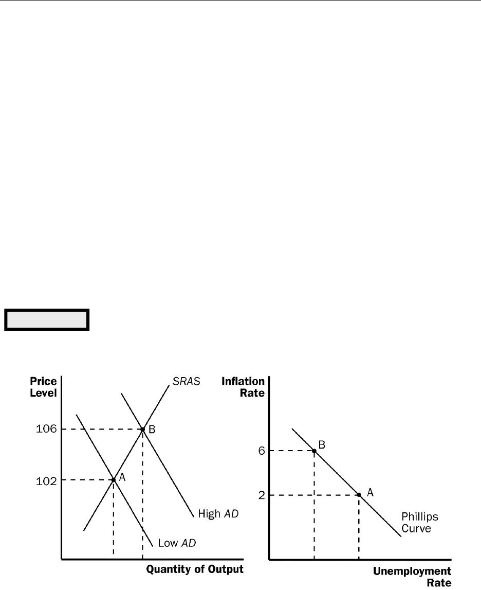
Figure 1
Show how the Phillips curve is derived from the aggregate
demand/aggregate supply model step by step. This graph is dierent from
all the other graphs that they have drawn in macroeconomics, because it
Chapter 35/The Short-Run Trade-o between Ination and Unemployment ❖ 593
3. Example: The price level is 100 (measured by the Consumer Price Index) in the
year 2020. There are two possible changes in the economy for the year 2021: a
low level of aggregate demand or a high level of aggregate demand.
a. If the economy experiences a low level of aggregate demand, we would be at
a short-run equilibrium like point A. This point also corresponds with point A on
the Phillips curve. Note that when aggregate demand is low, the ination rate
is relatively low and the unemployment rate is relatively high.
b. If the economy experiences a high level of aggregate demand, we would be at
a short-run equilibrium like point B. This point also corresponds with point B
on the Phillips curve. Note that when aggregate demand is high, the ination
rate is relatively high and the unemployment rate is relatively low.
4. Because monetary and @scal policies both shift the aggregate-demand curve,
these policies can move the economy along the Phillips curve.
© 2018 Cengage Learning®. May not be scanned, copied or duplicated, or posted to a publicly accessible website,
in whole or in part, except for use as permitted in a license distributed with a certain product or service or otherwise
on a password-protected website or school-approved learning management system for classroom use.
Figure 2
594 ❖ Chapter 35/The Short-Run Trade-o between Ination and Unemployment
a. Increases in the money supply, increases in government spending, or
decreases in taxes all increase aggregate demand and move the economy to
a point on the Phillips curve with lower unemployment and higher ination.
b. Decreases in the money supply, decreases in government spending, or
increases in taxes all lower aggregate demand and move the economy to a
point on the Phillips curve with higher unemployment and lower ination.
II. Shifts in the Phillips Curve: The Role of Expectations
A. The Long-Run Phillips Curve
1. In 1968, economist Milton Friedman argued that monetary policy is only able to
choose a combination of unemployment and ination for a short period of time. At
the same time, economist Edmund Phelps wrote a paper suggesting the same
thing.
2. In the long run, monetary growth has no real eects. This implies that it cannot
aect the factors that determine the economy’s long-run unemployment rate.
© 2018 Cengage Learning®. May not be scanned, copied or duplicated, or posted to a publicly accessible website,
in whole or in part, except for use as permitted in a license distributed with a certain product or service or otherwise
on a password-protected website or school-approved learning management system for classroom use.
Figure 3
Chapter 35/The Short-Run Trade-o between Ination and Unemployment ❖ 595
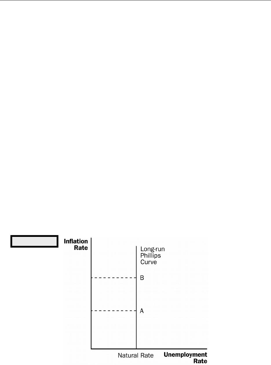
3. Thus, in the long run, we would not expect there to be a relationship between
unemployment and ination. This must mean that, in the long run, the Phillips
curve is vertical.
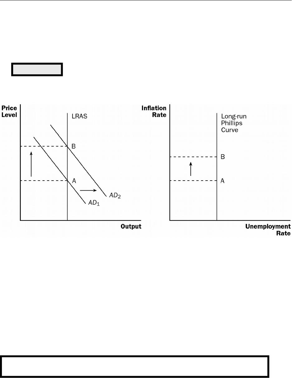
4. The vertical Phillips curve occurs because, in the long run, the aggregate supply
curve is vertical as well. Thus, increases in aggregate demand lead only to
changes in the price level and have no eect on the economy’s level of output.
Thus, in the long run, unemployment will not change when aggregate demand
changes, but ination will.
5. The long-run aggregate-supply curve occurs at the economy’s natural level of
output. This means that the long-run Phillips curve occurs at the natural rate of
unemployment.
B. The Meaning of “Natural”
© 2018 Cengage Learning®. May not be scanned, copied or duplicated, or posted to a publicly accessible website,
in whole or in part, except for use as permitted in a license distributed with a certain product or service or otherwise
on a password-protected website or school-approved learning management system for classroom use.
Figure 4
You may want to review what is meant by the “natural rate” of
unemployment.

596 ❖ Chapter 35/The Short-Run Trade-o between Ination and Unemployment
1. Friedman and Phelps considered the natural rate of unemployment to be the rate
toward which the economy gravitates in the long run.
2. The natural rate of unemployment may not be the socially desirable rate of
unemployment.
3. The natural rate of unemployment may change over time.
C. Reconciling Theory and Evidence
1. The conclusion of Friedman and Phelps that there is no long-run trade-o between
ination and unemployment was based on theory, while the correlation between
ination and unemployment found by Phillips, Samuelson, and Solow was based
on actual evidence.
2. Friedman and Phelps believed that an inverse relationship between ination and
unemployment exists in the short run.
3. The long-run aggregate-supply curve is vertical, indicating that the price level
does not inuence output in the long run.
4. But, the short-run aggregate-supply curve is upward sloping because of
misperceptions about relative prices, sticky wages, and sticky prices. These
perceptions, wages, and prices adjust over time, so that the positive relationship
between the price level and the quantity of goods and services supplied occurs
only in the short run.
5. This same logic applies to the Phillips curve. The trade-o between ination and
unemployment holds only in the short run.
6. The expected level of ination is an important factor in understanding the
dierence between the long-run and the short-run Phillips curves. Expected
ination measures how much people expect the overall price level to change.
© 2018 Cengage Learning®. May not be scanned, copied or duplicated, or posted to a publicly accessible website,
in whole or in part, except for use as permitted in a license distributed with a certain product or service or otherwise
on a password-protected website or school-approved learning management system for classroom use.
Chapter 35/The Short-Run Trade-o between Ination and Unemployment ❖ 597
7. The expected rate of ination is one variable that determines the position of the
short-run aggregate-supply curve. This is true because the expected price level
aects the perceptions of relative prices that people form and the wages and
prices that they set.
8. In the short run, expectations are somewhat @xed. Thus, when the Fed increases
the money supply, aggregate demand increases along the upward sloping
short-run aggregate-supply curve. Output grows (unemployment falls) and the
price level rises (ination increases).
9. Eventually, however, people will respond by changing their expectations of the
price level. Speci@cally, they will begin expecting a higher rate of ination.
D. The Short-Run Phillips Curve
1. We can relate the actual unemployment rate to the natural rate of
unemployment, the actual ination rate, and the expected ination rate using the
following equation:
a. Because expected ination is already given in the short run, higher actual
ination leads to lower unemployment.
b. How much unemployment changes in response to a change in ination is
determined by the variable a, which is related to the slope of the short-run
aggregate-supply curve.
© 2018 Cengage Learning®. May not be scanned, copied or duplicated, or posted to a publicly accessible website,
in whole or in part, except for use as permitted in a license distributed with a certain product or service or otherwise
on a password-protected website or school-approved learning management system for classroom use.
Be sure to discuss why actual ination always equals expected ination
along the long-run Phillips curve.
unemp. rate natural rate (actual ination expected ination)a= – –
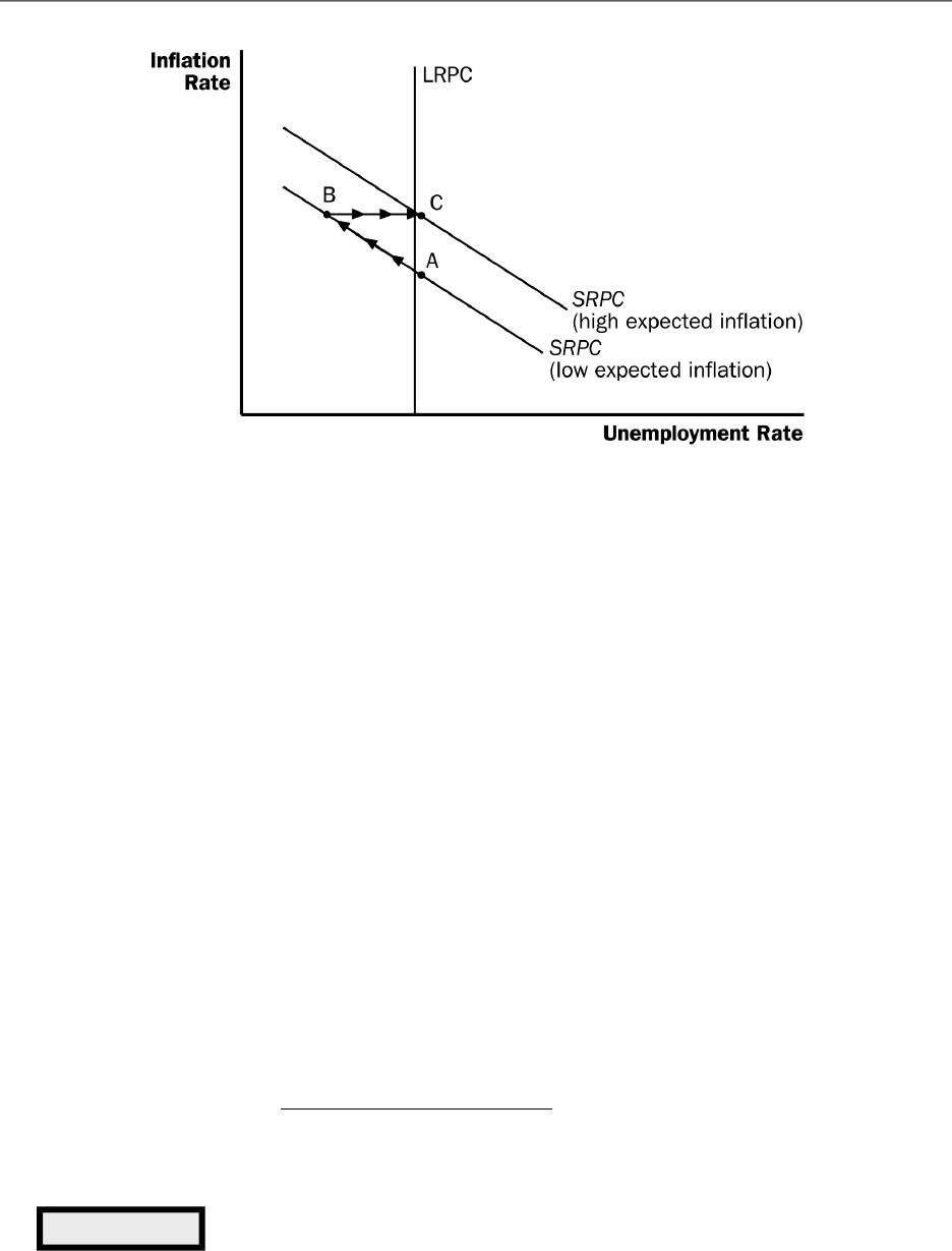
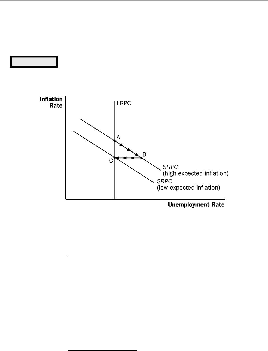
Figure 5
598 ❖ Chapter 35/The Short-Run Trade-o between Ination and Unemployment
2. If policymakers want to take advantage of the short-run trade-o between
unemployment and ination, it may lead to negative consequences.
a. Suppose the economy is at point A and policymakers wish to lower the
unemployment rate. Expansionary monetary policy or @scal policy is used to
shift aggregate demand to the right. The economy moves to point B, with a
lower unemployment rate and a higher rate of ination.
b. Over time, people get used to this new level of ination and raise their
expectations of ination. This leads to an upward shift of the short-run Phillips
curve. The economy ends up at point C, with a higher ination rate than at
point A, but the same level of unemployment.
E. The Natural Experiment for the Natural-Rate Hypothesis
1. De@nition of the natural-rate hypothesis: the claim that unemployment
eventually returns to its normal, or natural rate, regardless of the rate
of in0ation.
© 2018 Cengage Learning®. May not be scanned, copied or duplicated, or posted to a publicly accessible website,
in whole or in part, except for use as permitted in a license distributed with a certain product or service or otherwise
on a password-protected website or school-approved learning management system for classroom use.
Figure 6
Chapter 35/The Short-Run Trade-o between Ination and Unemployment ❖ 599
2. Figure 6 shows the unemployment and ination rates from 1961 to 1968. It is
easy to see the inverse relationship between these two variables.
3. Beginning in the late 1960s, the government followed policies that increased
aggregate demand.
a. Government spending rose because of the Vietnam War.
b. The Fed increased the money supply to try to keep interest rates down.
4. As a result of these policies, the ination rate remained fairly high. However, even
though ination remained high, unemployment did not remain low.
a. Figure 7 shows the unemployment and ination rates from 1961 to 1973. The
simple inverse relationship between these two variables began to disappear
around 1970.
b. Ination expectations adjusted to the higher rate of ination and the
unemployment rate returned to its natural rate of around 5% to 6%.
III. Shifts in the Phillips Curve: The Role of Supply Shocks
A. In 1974, OPEC increased the price of oil sharply. This increased the cost of producing
many goods and services and therefore resulted in higher prices.
1. De@nition of supply shock: an event that directly alters 4rms’ costs and
prices, shifting the economy’s aggregate-supply curve and thus the
Phillips curve.
© 2018 Cengage Learning®. May not be scanned, copied or duplicated, or posted to a publicly accessible website,
in whole or in part, except for use as permitted in a license distributed with a certain product or service or otherwise
on a password-protected website or school-approved learning management system for classroom use.
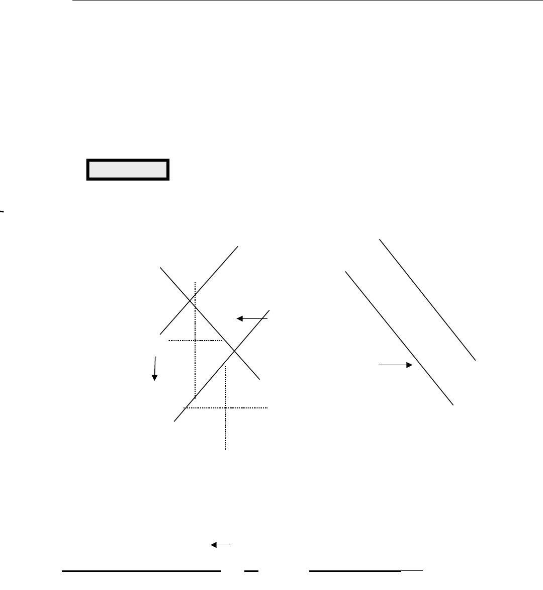
Figure 7
600 ❖ Chapter 35/The Short-Run Trade-o between Ination and Unemployment
2. Graphically, we could represent this supply shock as a shift in the short-run
aggregate-supply curve to the left.
3. The decrease in equilibrium output and the increase in the price level left the
economy with stagation.
B. Given this turn of events, policymakers are left with a less favorable short-run
trade-o between unemployment and ination.
© 2018 Cengage Learning®. May not be scanned, copied or duplicated, or posted to a publicly accessible website,
in whole or in part, except for use as permitted in a license distributed with a certain product or service or otherwise
on a password-protected website or school-approved learning management system for classroom use.
Price
Level
Outpu
t
Unemployment
Rate
In0atio
n
AD
AS1
AS2
PC2
PC1
Figure 8

Chapter 35/The Short-Run Trade-o between Ination and Unemployment ❖ 601
1. If they increase aggregate demand to @ght unemployment, they will raise
ination further.
2. If they lower aggregate demand to @ght ination, they will raise unemployment
further.
C. This less favorable trade-o between unemployment and ination can be shown by a
shift of the short-run Phillips curve. The shift may be permanent or temporary,
depending on how people adjust their expectations of ination.
D. During the 1970s, the Fed decided to accommodate the supply shock by increasing
the supply of money. This increased the level of expected ination. Figure 9 shows
ination and unemployment in the United States during the late 1970s and early
1980s.
IV. The Cost of Reducing Ination
A. The Sacri@ce Ratio
1. To reduce the ination rate, the Fed must follow contractionary monetary policy.
a. When the Fed slows the rate of growth of the money supply, aggregate
demand falls.
b. This reduces the level of output in the economy, increasing unemployment.
c. The economy moves from point A along the short-run Phillips curve to point B,
which has a lower ination rate but a higher unemployment rate.
© 2018 Cengage Learning®. May not be scanned, copied or duplicated, or posted to a publicly accessible website,
in whole or in part, except for use as permitted in a license distributed with a certain product or service or otherwise
on a password-protected website or school-approved learning management system for classroom use.
Figure 9
602 ❖ Chapter 35/The Short-Run Trade-o between Ination and Unemployment
d. Over time, people begin to adjust their ination expectations downward and
the short-run Phillips curve shifts. The economy moves from point B to point C,
where ination is lower and the unemployment rate is back to its natural rate.
2. Therefore, to reduce ination, the economy must suer through a period of high
unemployment and low output.
3. De@nition of sacri4ce ratio: the number of percentage points of annual
output lost in the process of reducing in0ation by one percentage point.
4. A typical estimate of the sacri@ce ratio is @ve. This implies that for each
percentage point ination is decreased, output falls by 5%.
B. Rational Expectations and the Possibility of Costless Disination
1. De@nition of rational expectations: the theory according to which people
optimally use all the information they have, including information about
government policies, when forecasting the future.
© 2018 Cengage Learning®. May not be scanned, copied or duplicated, or posted to a publicly accessible website,
in whole or in part, except for use as permitted in a license distributed with a certain product or service or otherwise
on a password-protected website or school-approved learning management system for classroom use.
Figure 10
Chapter 35/The Short-Run Trade-o between Ination and Unemployment ❖ 603
2. Proponents of rational expectations believe that when government policies
change, people alter their expectations about ination.
3. Therefore, if the government makes a credible commitment to a policy of low
ination, people would be rational enough to lower their expectations of ination
immediately. This implies that the short-run Phillips curve would shift quickly
without any extended period of high unemployment.
C. The Volcker Disination
1. Figure 11 shows the ination and unemployment rates that occurred while Paul
Volcker worked at reducing the level of ination during the 1980s.
2. As ination fell, unemployment rose. In fact, the United States experienced its
deepest recession since the Great Depression.
3. Some economists have oered this as proof that the idea of a costless disination
suggested by rational-expectations theorists is not possible. However, there are
two reasons why we might not want to reject the rational-expectations theory so
quickly.
a. The cost (in terms of lost output) of the Volcker disination was not as large as
many economists had predicted.
b. While Volcker promised that he would @ght ination, many people did not
believe him. Few people thought that ination would fall as quickly as it did;
this likely kept the short-run Phillips curve from shifting quickly.
D. The Greenspan Era
© 2018 Cengage Learning®. May not be scanned, copied or duplicated, or posted to a publicly accessible website,
in whole or in part, except for use as permitted in a license distributed with a certain product or service or otherwise
on a password-protected website or school-approved learning management system for classroom use.
Figure 11
Figure 12

604 ❖ Chapter 35/The Short-Run Trade-o between Ination and Unemployment
1. Figure 12 shows the ination and unemployment rate from 1984 to 2005, called
the Greenspan era because Alan Greenspan became the chair of the Federal
Reserve in 1987.
2. In 1986, OPEC’s agreement with its members broke down and oil prices fell. The
result of this favorable supply shock was a drop in both ination and
unemployment.
3. The rest of the 1990s witnessed a period of economic prosperity. Ination
gradually dropped, approaching zero by the end of the decade. Unemployment
also reached a low level, leading many people to believe that the natural rate of
unemployment had fallen.
4. The economy ran into problems in 2001 due to the end of the dot-com stock
market bubble, the 9-11 terrorist attacks, and corporate accounting scandals that
reduced aggregate demand. Unemployment rose as the economy experienced its
@rst recession in a decade.
5. But a combination of expansionary monetary and @scal policies helped end the
downturn, and by early 2005, the unemployment rate was close to the estimated
natural rate.
6. In 2005, President Bush nominated Ben Bernanke as the Fed chair.
E. A Financial Crisis Takes Us for a Ride Along the Phillips Curve
1. In his @rst couple of years as Fed chair, Bernanke faced some signi@cant
economic challenges.
a. One challenge arose from problems in the housing and @nancial markets.
b. The resulting @nancial crisis led to a large drop in aggregate demand and high
rates of unemployment.
© 2018 Cengage Learning®. May not be scanned, copied or duplicated, or posted to a publicly accessible website,
in whole or in part, except for use as permitted in a license distributed with a certain product or service or otherwise
on a password-protected website or school-approved learning management system for classroom use.

Chapter 35/The Short-Run Trade-o between Ination and Unemployment ❖ 605
c. Figure 13 shows the implications of these events for ination and
unemployment.
d. From 2007 to 2010, as the decline in aggregate demand raised unemployment
from below 5 percent to about 10 percent, it also reduced the ination rate
from about 3 percent to about 1 percent.
e. From 2010 to 2015, unemployment fell back to about 5 percent and the
ination rate remained between 1 percent and 2 percent.
f. In essence, the economy @rst rode down the Phillips curve and then rode back
up.
g. Note that expected ination and the position of the short-run Phillips curve
were relatively stable during this period.
© 2018 Cengage Learning®. May not be scanned, copied or duplicated, or posted to a publicly accessible website,
in whole or in part, except for use as permitted in a license distributed with a certain product or service or otherwise
on a password-protected website or school-approved learning management system for classroom use.
Figure 13