
WHAT’S NEW IN THE EIGHTH EDITION:
There is a new Ask the Experts feature on “Economic Stimulus” and a new question was
added to the Problems and Applications section.
LEARNING OBJECTIVES:
By the end of this chapter, students should understand:
the theory of liquidity preference as a short-run theory of the interest rate.
how monetary policy a ects interest rates and aggregate demand.
how “scal policy a ects interest rates and aggregate demand.
the debate over whether policymakers should try to stabilize the economy.
569
© 2018 Cengage Learning®. May not be scanned, copied or duplicated, or posted to a publicly accessible website,
in whole or in part, except for use as permitted in a license distributed with a certain product or service or otherwise
on a password-protected website or school-approved learning management system for classroom use.
34
THE INFLUENCE OF
MONETARY AND FISCAL
POLICY ON AGGREGATE
DEMAND

570 ❖ Chapter 34/The InDuence of Monetary and Fiscal Policy on Aggregate Demand
CONTEXT AND PURPOSE:
Chapter 34 is the second chapter in a three-chapter sequence that concentrates on
short-run Ductuations in the economy around its long-term trend. In Chapter 33, the model
of aggregate supply and aggregate demand is introduced. In Chapter 34, we see how the
government’s monetary and “scal policies a ect aggregate demand. In Chapter 35, we will
see some of the trade-o s between short-run and long-run objectives when we address the
relationship between inDation and unemployment.
The purpose of Chapter 34 is to address the short-run e ects of monetary and “scal
policies. In Chapter 33, we found that when aggregate demand or short-run aggregate
supply shifts, it causes Ductuations in output. As a result, policymakers sometimes try to
o set these shifts by shifting aggregate demand with monetary and “scal policy. Chapter 34
addresses the theory behind these policies and some of the shortcomings of stabilization
policy.
KEY POINTS:
In developing a theory of short-run economic Ductuations, Keynes proposed the theory of
liquidity preference to explain the determinants of the interest rate. According to this
theory, the interest rate adjusts to balance the supply and demand for money.
An increase in the price level raises money demand and increases the interest rate that
brings the money market into equilibrium. Because the interest rate represents the cost
of borrowing, a higher interest rate reduces investment and, thereby, the quantity of
goods and services demanded. The downward-sloping aggregate-demand curve
expresses this negative relationship between the price level and the quantity demanded.
Policymakers can inDuence aggregate demand with monetary policy. An increase in the
money supply reduces the equilibrium interest rate for any given price level. Because a
lower interest rate stimulates investment spending, the aggregate-demand curve shifts
to the right. Conversely, a decrease in the money supply raises the equilibrium interest
rate for any given price level and shifts the aggregate-demand curve to the left.
© 2018 Cengage Learning®. May not be scanned, copied or duplicated, or posted to a publicly accessible website,
in whole or in part, except for use as permitted in a license distributed with a certain product or service or otherwise
on a password-protected website or school-approved learning management system for classroom use.

Chapter 34/The InDuence of Monetary and Fiscal Policy on Aggregate Demand ❖ 571
Policymakers can also inDuence aggregate demand with “scal policy. An increase in
government purchases or a cut in taxes shifts the aggregate-demand curve to the right.
A decrease in government purchases or an increase in taxes shifts the
aggregate-demand curve to the left.
When the government alters spending or taxes, the resulting shift in aggregate demand
can be larger or smaller than the “scal change. The multiplier e ect tends to amplify the
e ects of “scal policy on aggregate demand. The crowding-out e ect tends to dampen
the e ects of “scal policy on aggregate demand.
Because monetary and “scal policy can inDuence aggregate demand, the government
sometimes uses these policy instruments in an attempt to stabilize the economy.
Economists disagree about how active the government should be in this e ort. According
to the advocates of active stabilization policy, changes in attitudes by households and
“rms shift aggregate demand; if the government does not respond, the result is
undesirable and unnecessary Ductuations in output and employment. According to critics
of active stabilization policy, monetary and “scal policy work with such long lags that
attempts at stabilizing the economy often end up being destabilizing.
CHAPTER OUTLINE:
I. How Monetary Policy InDuences Aggregate Demand
A. The aggregate-demand curve is downward sloping for three reasons.
© 2018 Cengage Learning®. May not be scanned, copied or duplicated, or posted to a publicly accessible website,
in whole or in part, except for use as permitted in a license distributed with a certain product or service or otherwise
on a password-protected website or school-approved learning management system for classroom use.
The e ects of monetary policy are easy to show graphically. Begin with
money supply, money demand, and an equilibrium interest rate. Show
how both an increase and a decrease in the money supply a ect interest
Students are very interested in the way in which the Fed changes interest
rates. Review what they learned about the Fed and its tools to change the
money supply.

572 ❖ Chapter 34/The InDuence of Monetary and Fiscal Policy on Aggregate Demand
1. The wealth e ect.
2. The interest-rate e ect.
3. The exchange-rate e ect.
B. All three e ects occur simultaneously, but are not of equal importance.
1. Because a household’s money holdings are a small part of total wealth, the
wealth e ect is the least important of the three.
2. Because imports and exports are a small fraction of U.S. GDP, the exchange-rate
e ect is also fairly small for the U.S. economy.
3. Thus, the most important reason for the downward-sloping aggregate-demand
curve is the interest-rate e ect.
C. De”nition of theory of liquidity preference: Keynes’s theory that the interest
rate adjusts to bring money supply and money demand into balance.
D. The Theory of Liquidity Preference
1. This theory is an explanation of the supply and demand for money and how they
relate to the interest rate.
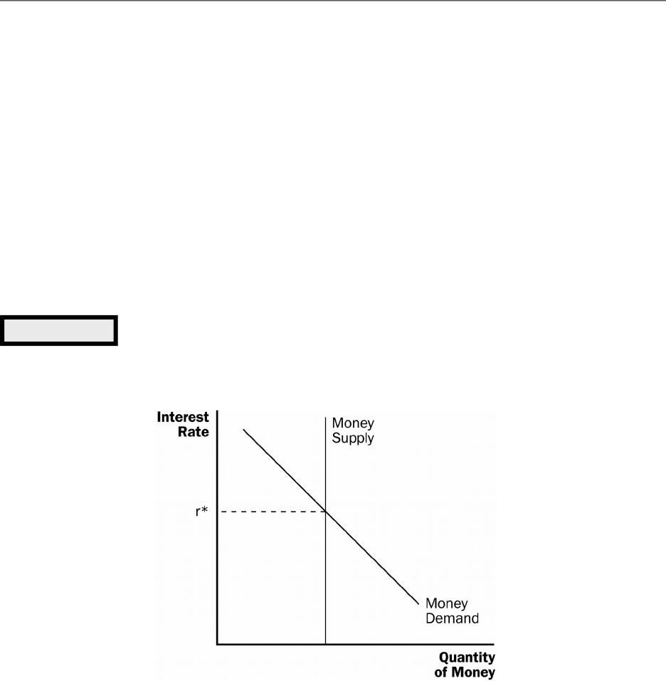
2. Money Supply
© 2018 Cengage Learning®. May not be scanned, copied or duplicated, or posted to a publicly accessible website,
in whole or in part, except for use as permitted in a license distributed with a certain product or service or otherwise
on a password-protected website or school-approved learning management system for classroom use.
Point out that when we discuss the “interest rate” we are discussing both
the nominal interest rate and the real interest rate because we are
assuming that they will move together. Remind the students of the Fisher
Chapter 34/The InDuence of Monetary and Fiscal Policy on Aggregate Demand ❖ 573
a. The money supply in the economy is controlled by the Federal Reserve.
b. The Fed can alter the supply of money using open market operations, changes
in the discount rate, and changes in reserve requirements.
c. Because the Fed can control the size of the money supply directly, the
quantity of money supplied does not depend on any other economic variables,
including the interest rate. Thus, the supply of money is represented by a
vertical supply curve.
© 2018 Cengage Learning®. May not be scanned, copied or duplicated, or posted to a publicly accessible website,
in whole or in part, except for use as permitted in a license distributed with a certain product or service or otherwise
on a password-protected website or school-approved learning management system for classroom use.
Figure 1

574 ❖ Chapter 34/The InDuence of Monetary and Fiscal Policy on Aggregate Demand
3. Money Demand
a. Any asset’s liquidity refers to the ease with which that asset can be converted
into a medium of exchange. Thus, money is the most liquid asset in the
economy.
b. The liquidity of money explains why people choose to hold it instead of other
assets that could earn them a higher return.
c. However, the return on other assets (the interest rate) is the opportunity cost
of holding money. All else being equal, as the interest rate rises, the quantity
of money demanded will fall. Therefore, the demand for money will be
downward sloping.
4. Equilibrium in the Money Market
a. The interest rate adjusts to bring money demand and money supply into
balance.
b. If the interest rate is higher than the equilibrium interest rate, the quantity of
money that people want to hold is less than the quantity that the Fed has
supplied. Thus, people will try to buy bonds or deposit funds in an
interest-bearing account. This increases the funds available for lending,
pushing interest rates down.
c. If the interest rate is lower than the equilibrium interest rate, the quantity of
money that people want to hold is greater than the quantity that the Fed has
supplied. Thus, people will try to sell bonds or withdraw funds from an
interest-bearing account. This decreases the funds available for lending,
pulling interest rates up.
E. FYI: Interest Rates in the Long Run and the Short Run
1. In an earlier chapter, we said that the interest rate adjusts to balance the supply
and demand for loanable funds.
© 2018 Cengage Learning®. May not be scanned, copied or duplicated, or posted to a publicly accessible website,
in whole or in part, except for use as permitted in a license distributed with a certain product or service or otherwise
on a password-protected website or school-approved learning management system for classroom use.

Chapter 34/The InDuence of Monetary and Fiscal Policy on Aggregate Demand ❖ 575
2. In this chapter, we proposed that the interest rate adjusts to balance the supply
and demand for money.
3. To understand how these two statements can both be true, we must discuss the
di erence between the short run and the long run.
4. In the long run, the economy’s level of output, the interest rate, and the price
level are determined by the following manner:
a. Output is determined by the levels of resources and technology available.
b. For any given level of output, the interest rate adjusts to balance the supply
and demand for loanable funds.
c. Given output and the interest rate, the price level adjusts to balance the
supply and demand for money. Changes in the supply of money lead to
proportionate changes in the price level.
5. In the short run, the economy’s level of output, the interest rate, and the price
level are determined by the following manner:
a. The price level is stuck at some level (based on previously formed
expectations) and is unresponsive to changes in economic conditions.
b. For any given price level, the interest rate adjusts to balance the supply and
demand for money.
c. The interest rate that balances the money market inDuences the quantity of
goods and services demanded and thus the level of output.
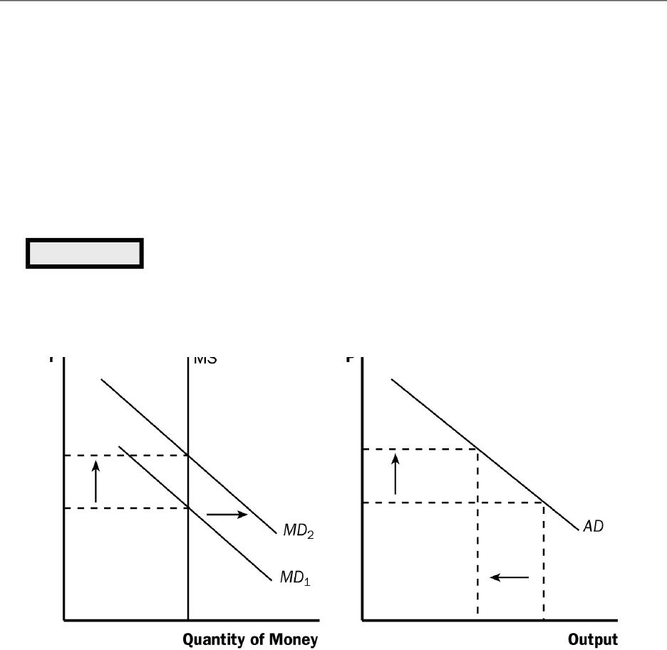
F. The Downward Slope of the Aggregate-Demand Curve
© 2018 Cengage Learning®. May not be scanned, copied or duplicated, or posted to a publicly accessible website,
in whole or in part, except for use as permitted in a license distributed with a certain product or service or otherwise
on a password-protected website or school-approved learning management system for classroom use.
576 ❖ Chapter 34/The InDuence of Monetary and Fiscal Policy on Aggregate Demand
1. When the price level increases, the quantity of money that people need to hold
becomes larger. Thus, an increase in the price level leads to an increase in the
demand for money, shifting the money demand curve to the right.
2. For a “xed money supply, the interest rate must rise to balance the supply and
demand for money.
3. At a higher interest rate, the cost of borrowing and the return on saving both
increase. Thus, consumers will choose to spend less and will be less likely to
invest in new housing. Firms will be less likely to borrow funds for new equipment
or structures. In short, the quantity of goods and services purchased in the
economy will fall.
4. As the price level increases, the quantity of goods and services demanded falls.
This is Keynes’s interest-rate e ect.
© 2018 Cengage Learning®. May not be scanned, copied or duplicated, or posted to a publicly accessible website,
in whole or in part, except for use as permitted in a license distributed with a certain product or service or otherwise
on a password-protected website or school-approved learning management system for classroom use.
Figure 2
Chapter 34/The InDuence of Monetary and Fiscal Policy on Aggregate Demand ❖ 577
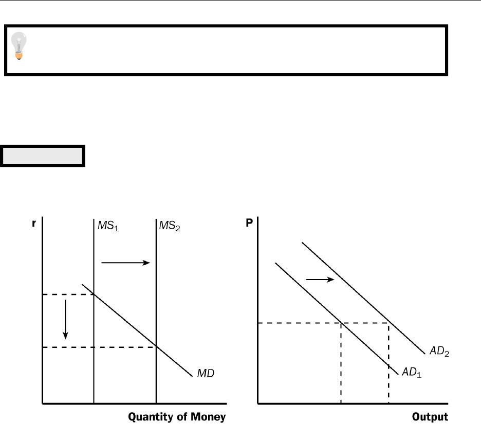
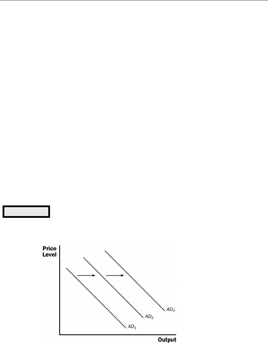
G. Changes in the Money Supply
1. Example: The Fed buys government bonds in open-market operations.
2. This will increase the supply of money, shifting the money supply curve to the
right. The equilibrium interest rate will fall.
3. The lower interest rate reduces the cost of borrowing and the return to saving.
This encourages households to increase their consumption and desire to invest in
new housing. Firms will also increase investment, building new factories and
purchasing new equipment.
4. The quantity of goods and services demanded will rise at every price level,
shifting the aggregate-demand curve to the right.
© 2018 Cengage Learning®. May not be scanned, copied or duplicated, or posted to a publicly accessible website,
in whole or in part, except for use as permitted in a license distributed with a certain product or service or otherwise
on a password-protected website or school-approved learning management system for classroom use.
Go through the example above in reverse as well. Make sure that students
understand that a decline in the price level will lead to a drop in money
demand and the interest rate and that this will cause a rise in aggregate
Figure 3

578 ❖ Chapter 34/The InDuence of Monetary and Fiscal Policy on Aggregate Demand
5. Thus, a monetary injection by the Fed increases the money supply, leading to a
lower interest rate, and a larger quantity of goods and services demanded.
H. The Role of Interest-Rate Targets in Fed Policy
1. In recent years, the Fed has conducted policy by setting a target for the federal
funds rate (the interest rate that banks charge one another for short-term loans).
© 2018 Cengage Learning®. May not be scanned, copied or duplicated, or posted to a publicly accessible website,
in whole or in part, except for use as permitted in a license distributed with a certain product or service or otherwise
on a password-protected website or school-approved learning management system for classroom use.
Show students that the Fed can target either the money supply or the
interest rate, but not both.
Point out the circumstances under which the Fed is likely to increase the
money supply. Then, discuss the circumstances under which the Fed is
likely to decrease the money supply. Discuss the short- and long-run
ALTERNATIVE CLASSROOM EXAMPLE:
Suppose the Fed sells government bonds in the open market. The following would
occur:
1. The supply of money will decrease, shifting the money supply curve to the left.
2. The equilibrium interest rate will rise, raising the cost of borrowing and the
Chapter 34/The InDuence of Monetary and Fiscal Policy on Aggregate Demand ❖ 579
a. The target is re-evaluated every six weeks when the Federal Open Market
Committee meets.
b. The Fed has chosen to use this interest rate as a target in part because the
money supply is diOcult to measure with suOcient precision.
2. Because changes in the money supply lead to changes in interest rates, monetary
policy can be described either in terms of the money supply or in terms of the
interest rate.
I. Case Study: Why the Fed Watches the Stock Market (and Vice Versa)
1. A booming stock market expands the aggregate demand for goods and services.
a. When the stock market booms, households become wealthier, and this
increased wealth stimulates consumer spending.
b. Increases in stock prices make it attractive for “rms to issue new shares of
stock and this increases investment spending.
2. Because one of the Fed’s goals is to stabilize aggregate demand, the Fed may
respond to a booming stock market by keeping the supply of money lower and
raising interest rates. The opposite would hold true if the stock market would fall.
3. Stock market participants also keep an eye on the Fed’s policy plans. When the
Fed lowers the money supply, it makes stocks less attractive because alternative
assets (such as bonds) pay higher interest rates. Also, higher interest rates may
lower the expected pro”tability of “rms.
© 2018 Cengage Learning®. May not be scanned, copied or duplicated, or posted to a publicly accessible website,
in whole or in part, except for use as permitted in a license distributed with a certain product or service or otherwise
on a password-protected website or school-approved learning management system for classroom use.
Make sure that you point out to students that, while the media describes
the actions of the Federal Reserve as “changing interest rates,” they
instead could be described as “changing the money supply.”

580 ❖ Chapter 34/The InDuence of Monetary and Fiscal Policy on Aggregate Demand
J. FYI: The Zero Lower Bound
1. What if the Fed’s target interest rate is already close to zero?
2. Some economists describe this situation as a liquidity trap.
a. Nominal interest rates cannot fall much below zero.
b. Expansionary monetary policy might not have any e ect.
3. Other economists are less concerned with this situation.
a. The central bank could alter inDationary expectations.
b. The Fed could also use other “nancial instruments in open market operations.
II. How Fiscal Policy InDuences Aggregate Demand
A. De”nition of 0scal policy: the setting of the level of government spending
and taxation by government policymakers.
B. Changes in Government Purchases
1. When the government changes the level of its purchases, it inDuences aggregate
demand directly. An increase in government purchases shifts the
aggregate-demand curve to the right, while a decrease in government purchases
shifts the aggregate-demand curve to the left.
2. There are two macroeconomic e ects that cause the size of the shift in the
aggregate-demand curve to be di erent from the change in the level of
© 2018 Cengage Learning®. May not be scanned, copied or duplicated, or posted to a publicly accessible website,
in whole or in part, except for use as permitted in a license distributed with a certain product or service or otherwise
on a password-protected website or school-approved learning management system for classroom use.
Chapter 34/The InDuence of Monetary and Fiscal Policy on Aggregate Demand ❖ 581
government purchases. They are called the multiplier e ect and the crowding-out
e ect.
C. The Multiplier E ect
1. Suppose that the government buys a product from a company.
a. The immediate impact of the purchase is to raise pro”ts and employment at
that “rm.
b. As a result, owners and workers at this “rm will see an increase in income,
and will therefore likely increase their own consumption.
c. Thus, total spending rises by more than the increase in government
purchases.
© 2018 Cengage Learning®. May not be scanned, copied or duplicated, or posted to a publicly accessible website,
in whole or in part, except for use as permitted in a license distributed with a certain product or service or otherwise
on a password-protected website or school-approved learning management system for classroom use.
Figure 4

582 ❖ Chapter 34/The InDuence of Monetary and Fiscal Policy on Aggregate Demand
2. De”nition of multiplier e4ect: the additional shifts in aggregate demand
that result when expansionary 0scal policy increases income and
thereby increases consumer spending.
3. The multiplier e ect continues even after the “rst round.
a. When consumers spend part of their additional income, it provides additional
income for other consumers.
b. These consumers then spend some of this additional income, raising the
incomes of yet another group of consumers.
4. A Formula for the Spending Multiplier
a. The marginal propensity to consume (MPC ) is the fraction of extra income
that a household consumes rather than saves.
b. Example: The government spends $20 billion on new planes. Assume that
MPC = 3/4.
c. Incomes will increase by $20 billion, so consumption will rise by MPC × $20
billion. The second increase in consumption will be equal to MPC × (MPC ×
$20 billion) or MPC 2 × $20 billion.
d. To “nd the total impact on the demand for goods and services, we add up all
of these e ects:
Change in government purchases = $20 billion
First change in consumption = MPC × $20 billion
Second change in consumption = MPC2 × $20 billion
Third change in consumption = MPC3 × $20 billion
· ·
© 2018 Cengage Learning®. May not be scanned, copied or duplicated, or posted to a publicly accessible website,
in whole or in part, except for use as permitted in a license distributed with a certain product or service or otherwise
on a password-protected website or school-approved learning management system for classroom use.
Chapter 34/The InDuence of Monetary and Fiscal Policy on Aggregate Demand ❖ 583
· ·
· ·
Total Change = (1 + MPC + MPC 2 + MPC 3 + . . .) × $20 billion
e. This means that the multiplier can be written as:
Multiplier = (1 + MPC + MPC 2 + MPC 3 + . . .).
f. Because this expression is an in”nite geometric series, it also can be written
as:
g. Note that the size of the multiplier depends on the marginal propensity to
consume.
5. Other Applications of the Multiplier E ect
a. The multiplier e ect applies to any event that alters spending on any
component of GDP (consumption, investment, government purchases, or net
exports).
b. Examples include a reduction in net exports due to a recession in another
country or a stock market boom that raises consumption.
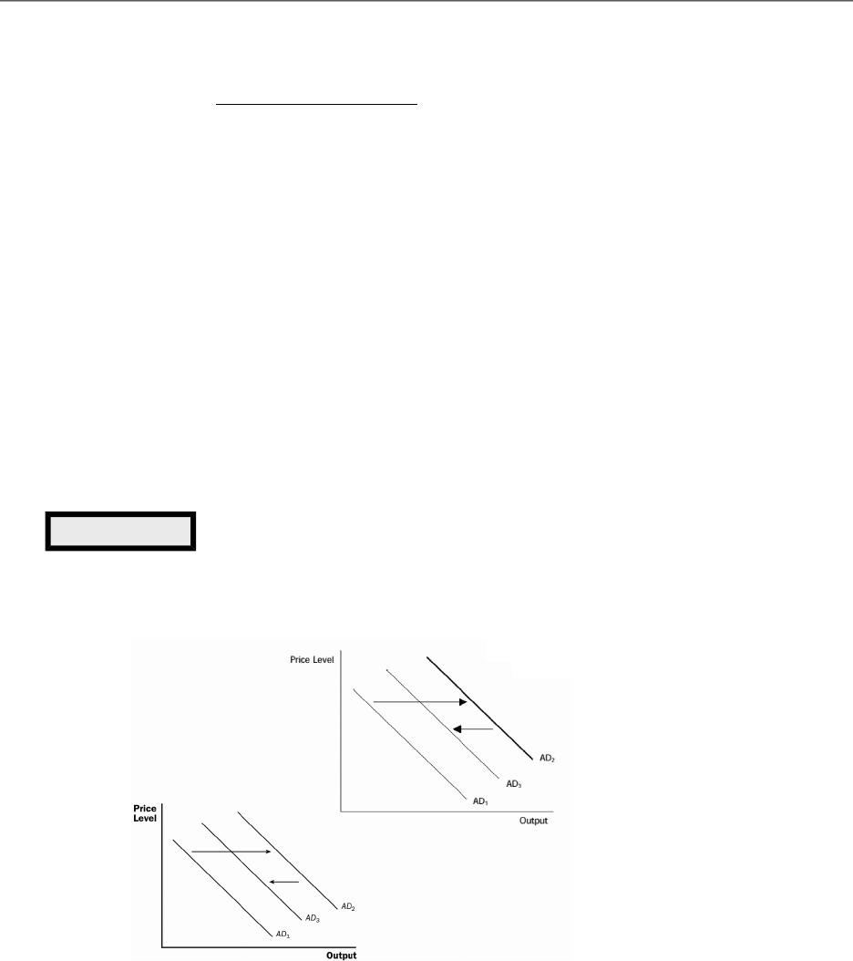
D. The Crowding-Out E ect
1. The crowding-out e ect works in the opposite direction.
© 2018 Cengage Learning®. May not be scanned, copied or duplicated, or posted to a publicly accessible website,
in whole or in part, except for use as permitted in a license distributed with a certain product or service or otherwise
on a password-protected website or school-approved learning management system for classroom use.
multiplier 1/(1 )MPC= –
584 ❖ Chapter 34/The InDuence of Monetary and Fiscal Policy on Aggregate Demand
2. De”nition of crowding-out e4ect: the o4set in aggregate demand that
results when expansionary 0scal policy raises the interest rate and
thereby reduces investment spending.
3. As we discussed earlier, when the government buys a product from a company,
the immediate impact of the purchase is to raise pro”ts and employment at that
“rm. As a result, owners and workers at this “rm will see an increase in income,
and will therefore likely increase their own consumption.
4. If consumers want to purchase more goods and services, they will need to
increase their holdings of money. This shifts the demand for money to the right,
pushing up the interest rate.
5. The higher interest rate raises the cost of borrowing and the return to saving. This
discourages households from spending their incomes for new consumption or
investing in new housing. Firms will also decrease investment, choosing not to
build new factories or purchase new equipment.
© 2018 Cengage Learning®. May not be scanned, copied or duplicated, or posted to a publicly accessible website,
in whole or in part, except for use as permitted in a license distributed with a certain product or service or otherwise
on a password-protected website or school-approved learning management system for classroom use.
Figure 5

Chapter 34/The InDuence of Monetary and Fiscal Policy on Aggregate Demand ❖ 585
6. Thus, even though the increase in government purchases shifts the
aggregate-demand curve to the right, this fall in consumption and investment will
pull aggregate demand back toward the left. Thus, aggregate demand increases
by less than the increase in government purchases.
7. Therefore, when the government increases its purchases by $X, the aggregate
demand for goods and services could rise by more or less than $X, depending on
the sizes of the multiplier and crowding-out e ects.
a. If the multiplier e ect is greater than the crowding-out e ect, aggregate
demand will rise by more than $X.
b. If the multiplier e ect is less than the crowding-out e ect, aggregate demand
will rise by less than $X.
E. Changes in Taxes
1. Changes in taxes a ect a household’s take-home pay.
a. If the government reduces taxes, households will likely spend some of this
extra income, shifting the aggregate-demand curve to the right.
b. If the government raises taxes, household spending will fall, shifting the
aggregate-demand curve to the left.
2. The size of the shift in the aggregate-demand curve will also depend on the sizes
of the multiplier and crowding-out e ects.
a. When the government lowers taxes and consumption increases, earnings and
pro“ts rise, which further stimulate consumer spending. This is the multiplier
e ect.
© 2018 Cengage Learning®. May not be scanned, copied or duplicated, or posted to a publicly accessible website,
in whole or in part, except for use as permitted in a license distributed with a certain product or service or otherwise
on a password-protected website or school-approved learning management system for classroom use.

586 ❖ Chapter 34/The InDuence of Monetary and Fiscal Policy on Aggregate Demand
b. Higher incomes lead to greater spending, which means a higher demand for
money. Interest rates rise and investment spending falls. This is the
crowding-out e ect.
3. Another important determinant of the size of the shift in aggregate demand due
to a change in taxes is whether people believe that the tax change is permanent
or temporary. A permanent tax change will have a larger e ect on aggregate
demand than a temporary one.
F. FYI: How Fiscal Policy Might A-ect Aggregate Supply
1. Because people respond to incentives, a decrease in tax rates may cause
individuals to work more, because they get to keep more of what they earn. If this
occurs, the aggregate-supply curve would increase (shift to the right).
2. Changes in government purchases may also a ect supply. If the government
increases spending on capital projects or education, the productive ability of the
economy is enhanced, shifting aggregate supply to the right.
III. Using Policy to Stabilize the Economy
A. The Case for Active Stabilization Policy
1. Example: The government raises taxes, lowering aggregate demand (shifting the
curve to the left).
a. The Fed can o set this government action by increasing the money supply.
b. This would lower interest rates and boost spending, shifting the
aggregate-demand curve back to the right.
© 2018 Cengage Learning®. May not be scanned, copied or duplicated, or posted to a publicly accessible website,
in whole or in part, except for use as permitted in a license distributed with a certain product or service or otherwise
on a password-protected website or school-approved learning management system for classroom use.

Chapter 34/The InDuence of Monetary and Fiscal Policy on Aggregate Demand ❖ 587
2. Policy instruments are often used in this manner to stabilize demand. Economic
stabilization has been an explicit goal of U.S. policy since the Employment Act of
1946.
a. One implication of the Employment Act is that the government should avoid
being the cause of economic Ductuations.
b. The second implication of the Employment Act is that the government should
respond to changes in the private economy in order to stabilize aggregate
demand.
3. The Employment Act occurred in response to a book by John Maynard Keynes, an
economist who emphasized the important role of aggregate demand in explaining
short-run Ductuations in the economy.
4. Keynes also felt strongly that the government should stimulate aggregate
demand whenever necessary to keep the economy at full employment.
a. Keynes argued that aggregate demand responds strongly to pessimism and
optimism. When consumers are pessimistic, aggregate demand is low, output
is low, and unemployment is increased. When consumers are optimistic,
aggregate demand is high, output is high, and unemployment is lowered.
b. It is possible for the government to adjust monetary and “scal policy in
response to optimistic or pessimistic views. This helps stabilize aggregate
demand, keeping output stable at full employment.
5. Case Study: Keynesians in the White House
a. In 1961, President Kennedy pushed for a tax cut to stimulate aggregate
demand. Several of his economic advisers were followers of Keynes.
b. In 2009, President Obama pushed for a stimulus bill that included several
increases in government spending.
© 2018 Cengage Learning®. May not be scanned, copied or duplicated, or posted to a publicly accessible website,
in whole or in part, except for use as permitted in a license distributed with a certain product or service or otherwise
on a password-protected website or school-approved learning management system for classroom use.

588 ❖ Chapter 34/The InDuence of Monetary and Fiscal Policy on Aggregate Demand
6. Ask the Experts: Economic Stimulus
a. 97 percent of economic experts agree that the U.S. unemployment rate was
lower at the end of 2010 than would have been without the 2009 stimulus bill.
b. 75 percent of economic experts agree that the bene”ts will outweigh the costs
of the 2009 stimulus bill, while 6 percent disagree and 19 percent are
uncertain.
7. In the News: How Large is the Fiscal Policy Multiplier?
a. During the large economic recession of 2008–2009, many governments tried
using expansionary “scal policy to stimulate aggregate demand.
b. This article from The Economist describes the debate over the estimated
e ects of these policies.
B. The Case against Active Stabilization Policy
1. Some economists believe that “scal and monetary policy tools should only be
used to help the economy achieve long-run goals, such as low inDation and rapid
economic growth.
2. The primary argument against active policy is that these policy tools may a ect
the economy with a long lag.
a. With monetary policy, the change in money supply leads to a change in
interest rates. This change in interest rates a ects investment spending.
However, investment decisions are usually made well in advance, so the
e ects from changes in investment will not likely be felt in the economy very
quickly.
b. The lag in “scal policy is generally due to the political process. Changes in
spending and taxes must be approved by both the House and the Senate
(after going through committees in both houses).
© 2018 Cengage Learning®. May not be scanned, copied or duplicated, or posted to a publicly accessible website,
in whole or in part, except for use as permitted in a license distributed with a certain product or service or otherwise
on a password-protected website or school-approved learning management system for classroom use.

Chapter 34/The InDuence of Monetary and Fiscal Policy on Aggregate Demand ❖ 589
3. By the time these policies take e ect, the condition of the economy may have
changed. This could lead to even larger problems.
C. Automatic Stabilizers
1. De”nition of automatic stabilizers: changes in 0scal policy that stimulate
aggregate demand when the economy goes into a recession without
policymakers having to take any deliberate action.
2. The most important automatic stabilizer is the tax system.
a. When the economy falls into a recession, incomes and pro”ts fall.
b. The personal income tax depends on the level of households’ incomes and the
corporate income tax depends on the level of “rm pro”ts.
c. This implies that the government’s tax revenue falls during a recession. This
tax cut stimulates aggregate demand and reduces the magnitude of this
economic downturn.
3. Some government spending is also an automatic stabilizer.
a. More individuals become eligible for transfer payments during a recession.
b. These transfer payments provide additional income to recipients, stimulating
spending.
c. Thus, just like the tax system, our system of transfer payments helps to
reduce the size of short-run economic Ductuations.
© 2018 Cengage Learning®. May not be scanned, copied or duplicated, or posted to a publicly accessible website,
in whole or in part, except for use as permitted in a license distributed with a certain product or service or otherwise
on a password-protected website or school-approved learning management system for classroom use.

590 ❖ Chapter 34/The InDuence of Monetary and Fiscal Policy on Aggregate Demand
© 2018 Cengage Learning®. May not be scanned, copied or duplicated, or posted to a publicly accessible website,
in whole or in part, except for use as permitted in a license distributed with a certain product or service or otherwise
on a password-protected website or school-approved learning management system for classroom use.