
WHAT’S NEW IN THE EIGHTH EDITION:
There is an updated discussion of the Great Recession and its aftermath including a new In
the News feature on “Lingering Fears from the Great Recession.”
LEARNING OBJECTIVES:
By the end of this chapter, students should understand:
three key facts about short-run economic !uctuations.
how the economy in the short run di”ers from the economy in the long run.
how to use the model of aggregate demand and aggregate supply to explain economic
!uctuations.
539
© 2018 Cengage Learning®. May not be scanned, copied or duplicated, or posted to a publicly accessible website,
in whole or in part, except for use as permitted in a license distributed with a certain product or service or otherwise
on a password-protected website or school-approved learning management system for classroom use.
33 AGGREGATE DEMAND
AND AGGREGATE
SUPPLY

540 ❖ Chapter 33/Aggregate Demand and Aggregate Supply
how shifts in either aggregate demand or aggregate supply can cause booms and
recessions.
CONTEXT AND PURPOSE:
To this point, our study of macroeconomic theory has concentrated on the behavior of the
economy in the long run. Chapters 33 through 35 now focus on short-run !uctuations in the
economy around its long-term trend. Chapter 33 introduces aggregate demand and
aggregate supply and shows how shifts in these curves can cause recessions. Chapter 34
focuses on how policymakers use the tools of monetary and =scal policy to in!uence
aggregate demand. Chapter 35 addresses the relationship between in!ation and
unemployment.
The purpose of Chapter 33 is to develop the model economists use to analyze the
economy’s short-run !uctuations—the model of aggregate demand and aggregate supply.
Students will learn about some of the sources for shifts in the aggregate-demand curve and
the aggregate-supply curve and how these shifts can cause recessions. This chapter also
introduces actions policymakers might undertake to o”set recessions.
KEY POINTS:
All societies experience short-run economic !uctuations around long-run trends. These
!uctuations are irregular and largely unpredictable. When recessions occur, real GDP and
other measures of income, spending, and production fall, while unemployment rises.
Classical economic theory is based on the assumption that nominal variables such as the
money supply and the price level do not in!uence real variables such as output and
employment. Most economists believe that this assumption is accurate in the long run
but not in the short run. Economists analyze short-run economic !uctuations using the
model of aggregate demand and aggregate supply. According to this model, the output
of goods and services and the overall level of prices adjust to balance aggregate demand
and aggregate supply.
The aggregate-demand curve slopes downward for three reasons. The =rst is the wealth
e”ect: A lower price level raises the real value of households’ money holdings, which
© 2018 Cengage Learning®. May not be scanned, copied or duplicated, or posted to a publicly accessible website,
in whole or in part, except for use as permitted in a license distributed with a certain product or service or otherwise
on a password-protected website or school-approved learning management system for classroom use.

Chapter 33/Aggregate Demand and Aggregate Supply ❖ 541
stimulates consumer spending. The second is the interest-rate e”ect: A lower price level
reduces the quantity of money households demand; as households try to convert money
into interest-bearing assets, interest rates fall, which stimulates investment spending.
The third is the exchange-rate e”ect: As a lower price level reduces interest rates, the
dollar depreciates in the market for foreign-currency exchange, which stimulates net
exports.
Any event or policy that raises consumption, investment, government purchases, or net
exports at a given price level increases aggregate demand. Any event or policy that
reduces consumption, investment, government purchases, or net exports at a given
price level decreases aggregate demand.
The long-run aggregate-supply curve is vertical. In the long run, the quantity of goods
and services supplied depends on the economy’s labor, capital, natural resources, and
technology, but not on the overall level of prices.
Three theories have been proposed to explain the upward slope of the short-run
aggregate-supply curve. According to the sticky-wage theory, an unexpected fall in the
price level temporarily raises real wages, which induces =rms to reduce employment and
production. According to the sticky-price theory, an unexpected fall in the price level
leaves some =rms with prices that are temporarily too high, which reduces their sales
and causes them to cut back production. According to the misperceptions theory, an
unexpected fall in the price level leads suppliers to mistakenly believe that their relative
prices have fallen, which induces them to reduce production. All three theories imply that
output deviates from its natural level when the actual price level deviates from the price
level that people expected.
Events that alter the economy’s ability to produce output, such as changes in labor,
capital, natural resources, or technology, shift the short-run aggregate-supply curve (and
may shift the long-run aggregate-supply curve as well). In addition, the position of the
short-run aggregate-supply curve depends on the expected price level.
One possible cause of economic !uctuations is a shift in aggregate demand. When the
aggregate-demand curve shifts to the left, output and prices fall in the short run. Over
time, as a change in the expected price level causes perceptions, wages, and prices to
adjust, the short-run aggregate-supply curve shifts to the right. This shift returns the
economy to its natural level of output at a new, lower price level.
© 2018 Cengage Learning®. May not be scanned, copied or duplicated, or posted to a publicly accessible website,
in whole or in part, except for use as permitted in a license distributed with a certain product or service or otherwise
on a password-protected website or school-approved learning management system for classroom use.

542 ❖ Chapter 33/Aggregate Demand and Aggregate Supply
A second possible cause of economic !uctuations is a shift in aggregate supply. When
the short-run aggregate-supply curve shifts to the left, the e”ect is falling output and
rising prices―a combination called stag!ation. Over time, as perceptions, wages, and
prices adjust, the short-run aggregate-supply curve shifts back to the right, returning the
price level and output back to their original levels.
© 2018 Cengage Learning®. May not be scanned, copied or duplicated, or posted to a publicly accessible website,
in whole or in part, except for use as permitted in a license distributed with a certain product or service or otherwise
on a password-protected website or school-approved learning management system for classroom use.
Chapter 33/Aggregate Demand and Aggregate Supply ❖ 543
CHAPTER OUTLINE:
I. Economic activity !uctuates from year to year.
A. De=nition of recession: a period of declining real incomes and rising
unemployment.
B. De=nition of depression: a severe recession.
II. Three Key Facts about Economic Fluctuations
A. Fact 1: Economic Fluctuations Are Irregular and Unpredictable
1. Fluctuations in the economy are often called the business cycle.
2. Economic !uctuations correspond to changes in business conditions.
3. These !uctuations are not at all regular and are almost impossible to predict.
4. Panel (a) of Figure 1 shows real GDP since 1965. The shaded areas represent
recessions.
B. Fact 2: Most Macroeconomic Quantities Fluctuate Together
1. Real GDP is the variable that is most often used to examine short-run changes in
the economy.
© 2018 Cengage Learning®. May not be scanned, copied or duplicated, or posted to a publicly accessible website,
in whole or in part, except for use as permitted in a license distributed with a certain product or service or otherwise
on a password-protected website or school-approved learning management system for classroom use.
Figure 1

544 ❖ Chapter 33/Aggregate Demand and Aggregate Supply
2. However, most macroeconomic variables that measure some type of income,
spending, or production !uctuate closely together.
3. Panel (b) of Figure 1 shows how investment spending changes over the business
cycle. Note that investment spending falls during recessions just as real GDP
does.
C. Fact 3: As Output Falls, Unemployment Rises
1. Changes in the economy’s output level will have an e”ect on the economy’s
utilization of its labor force.
2. When =rms choose to produce a smaller amount of goods and services, they lay
o” workers, which increases the unemployment rate.
3. Panel (c) of Figure 1 shows how the unemployment rate changes over the
business cycle. Note that during recessions, unemployment generally rises. Note
also that the unemployment rate never approaches zero but instead !uctuates
around its natural rate of about 5% or 6%.
III. Explaining Short-Run Economic Fluctuations
A. The Assumptions of Classical Economics
1. The classical dichotomy is the separation of variables into real variables and
nominal variables.
2. According to classical theory, changes in the money supply only a”ect nominal
variables.
B. The Reality of Short-Run Fluctuations
© 2018 Cengage Learning®. May not be scanned, copied or duplicated, or posted to a publicly accessible website,
in whole or in part, except for use as permitted in a license distributed with a certain product or service or otherwise
on a password-protected website or school-approved learning management system for classroom use.

Chapter 33/Aggregate Demand and Aggregate Supply ❖ 545
1. Most economists believe that the classical theory describes the world in the long
run but not in the short run.
2. Beyond a period of several years, changes in the money supply a”ect prices and
other nominal variables, but do not a”ect real GDP, unemployment, or other real
variables.
3. However, when studying year-to-year !uctuations in the economy, the
assumption of monetary neutrality is not appropriate. In the short run, most real
and nominal variables are intertwined.
C. The Model of Aggregate Demand and Aggregate Supply
1. De=nition of model of aggregate demand and aggregate supply: the
model that most economists use to explain short-run 0uctuations in
economic activity around its long-run trend.
2. We can show this model using a graph.
a. The variable on the vertical axis is the average level of prices in the economy,
as measured by the CPI or the GDP de!ator.
b. The variable on the horizontal axis is the economy’s output of goods and
services, as measured by real GDP.
© 2018 Cengage Learning®. May not be scanned, copied or duplicated, or posted to a publicly accessible website,
in whole or in part, except for use as permitted in a license distributed with a certain product or service or otherwise
on a password-protected website or school-approved learning management system for classroom use.
Figure 2
Begin by reviewing demand, supply, and equilibrium. Make it clear that
the microeconomic variables of price and quantity can be aggregated into
a price level (measured by either the GDP de!ator or the Consumer Price
Index) and total output (real GDP).

546 ❖ Chapter 33/Aggregate Demand and Aggregate Supply
c. De=nition of aggregate-demand curve: a curve that shows the quantity
of goods and services that households, 3rms, and the government
want to buy at each price level.
d. De=nition of aggregate-supply curve: a curve that shows the quantity
of goods and services that 3rms choose to produce and sell at each
price level.
3. In this model, the price level and the quantity of output adjust to bring aggregate
demand and aggregate supply into balance.
IV. The Aggregate-Demand Curve
A. Why the Aggregate-Demand Curve Slopes Downward
© 2018 Cengage Learning®. May not be scanned, copied or duplicated, or posted to a publicly accessible website,
in whole or in part, except for use as permitted in a license distributed with a certain product or service or otherwise
on a password-protected website or school-approved learning management system for classroom use.
Chapter 33/Aggregate Demand and Aggregate Supply ❖ 547
1. Recall that GDP (Y ) is made up of four components: consumption (C ), investment
(I ), government purchases (G ), and net exports (NX ).
2. Each of the four components is a part of aggregate demand.
a. Government purchases are assumed to be =xed by policy.
b. This means that to understand why the aggregate-demand curve slopes
downward, we must understand how changes in the price level a”ect
consumption, investment, and net exports.
© 2018 Cengage Learning®. May not be scanned, copied or duplicated, or posted to a publicly accessible website,
in whole or in part, except for use as permitted in a license distributed with a certain product or service or otherwise
on a password-protected website or school-approved learning management system for classroom use.
Highlight the fact that all three of these e”ects begin with a decrease (or
increase) in the price level and end with an increase (decrease) in
aggregate quantity demanded.
You will likely need to remind students of the di”erence between changes
in quantity demanded (movements along the demand curve) and changes
in demand (shifts in the demand curve).
Y C I G NX= + + +
Figure 3

548 ❖ Chapter 33/Aggregate Demand and Aggregate Supply
3. The Price Level and Consumption: The Wealth E”ect
a. A decrease in the price level raises the real value of money and makes
consumers feel wealthier, which in turn encourages them to spend more.
b. The increase in consumer spending means a larger quantity of goods and
services demanded.
4. The Price Level and Investment: The Interest-Rate E”ect
a. The lower the price level, the less money households need to buy goods and
services.
b. When the price level falls, households try to reduce their holdings of money by
lending some out (either in =nancial markets or through =nancial
intermediaries).
c. As households try to convert some of their money into interest-bearing assets,
the interest rate will drop.
d. Lower interest rates encourage borrowing =rms to borrow more to invest in
new plants and equipment, and it encourages households to borrow more to
invest in new housing.
e. Thus, a lower price level reduces the interest rate, encourages greater
spending on investment goods, and therefore increases the quantity of goods
and services demanded.
5. The Price Level and Net Exports: The Exchange-Rate E”ect
a. A lower price level in the United States lowers the U.S. interest rate.
© 2018 Cengage Learning®. May not be scanned, copied or duplicated, or posted to a publicly accessible website,
in whole or in part, except for use as permitted in a license distributed with a certain product or service or otherwise
on a password-protected website or school-approved learning management system for classroom use.

Chapter 33/Aggregate Demand and Aggregate Supply ❖ 549
b. Some U.S. investors will seek higher returns by investing abroad, increasing
U.S. net capital out!ow.
c. The increase in net capital out!ow raises the supply of dollars, lowering the
real exchange rate.
d. U.S. goods become relatively cheaper to foreign goods. Exports rise, imports
fall, and net exports increase.
e. Therefore, when a fall in the U.S. price level causes U.S. interest rates to fall,
the real exchange rate depreciates, and U.S. net exports rise, thereby
increasing the quantity of goods and services demanded.
6. All three of these e”ects imply that, all else being equal, there is an inverse
relationship between the price level and the quantity of goods and services
demanded.
B. Why the Aggregate-Demand Curve Might Shift
1. Shifts Arising from Changes in Consumption
© 2018 Cengage Learning®. May not be scanned, copied or duplicated, or posted to a publicly accessible website,
in whole or in part, except for use as permitted in a license distributed with a certain product or service or otherwise
on a password-protected website or school-approved learning management system for classroom use.
Remind students that the aggregate-demand curve (like all demand
curves) is drawn assuming that everything else is held constant.
Get the students involved in suggesting factors that might shift the
aggregate- demand curve. Relate changes in aggregate demand to
changes in consumption, investment, government purchases, and net
exports. Show students that, if any of these four components of GDP
change (for reasons other than a change in the price level), the

550 ❖ Chapter 33/Aggregate Demand and Aggregate Supply
a. If Americans become more concerned with saving for retirement and reduce
current consumption, aggregate demand will shift to the left.
b. If the government cuts taxes, it encourages people to spend more, resulting in
a shift to the right in aggregate demand.
2. Shifts Arising from Changes in Investment
a. Suppose that the computer industry introduces a faster line of computers and
many =rms decide to invest in new computer systems. This will cause
aggregate demand to shift to the right.
b. If =rms become pessimistic about future business conditions, they may cut
back on investment spending, shifting aggregate demand to the left.
c. An investment tax credit increases the quantity of investment goods that
=rms demand, which shifts aggregate demand to the right.
d. An increase in the supply of money lowers the interest rate in the short run.
This leads to more investment spending, which causes aggregate demand to
shift to the right.
3. Shifts Arising from Changes in Government Purchases
a. If Congress decides to reduce purchases of new weapon systems, aggregate
demand will shift to the left.
b. If state governments decide to build more highways, aggregate demand will
shift to the right.
4. Shifts Arising from Changes in Net Exports
© 2018 Cengage Learning®. May not be scanned, copied or duplicated, or posted to a publicly accessible website,
in whole or in part, except for use as permitted in a license distributed with a certain product or service or otherwise
on a password-protected website or school-approved learning management system for classroom use.

Chapter 33/Aggregate Demand and Aggregate Supply ❖ 551
a. When Europe experiences a recession, it buys fewer American goods, which
lowers U.S. net exports at every price level. Aggregate demand for the U.S.
economy will shift to the left.
b. If the exchange rate of the U.S. dollar increases, U.S. goods become more
expensive to foreigners. Net exports fall and aggregate demand shifts to the
left.
V. The Aggregate-Supply Curve
A. The relationship between the price level and the quantity of goods and services
supplied depends on the time horizon being examined.
B. Why the Aggregate-Supply Curve Is Vertical in the Long Run
1. In the long run, an economy’s production of goods and services depends on its
supplies of resources along with the available production technology.
2. Because the price level does not a”ect these determinants of output in the long
run, the long-run aggregate-supply curve is vertical.
© 2018 Cengage Learning®. May not be scanned, copied or duplicated, or posted to a publicly accessible website,
in whole or in part, except for use as permitted in a license distributed with a certain product or service or otherwise
on a password-protected website or school-approved learning management system for classroom use.
Table 1
552 ❖ Chapter 33/Aggregate Demand and Aggregate Supply
3. The vertical long-run aggregate-supply curve is a graphical representation of the
classical dichotomy and monetary neutrality.
C. Why the Long-Run Aggregate-Supply Curve Might Shift
1. The position of the aggregate-supply curve occurs at an output level sometimes
referred to as potential output or full-employment output.
2. De=nition of natural level of output: the production of goods and services
that an economy achieves in the long run when unemployment is at its
natural rate.
3. Any change in the economy that alters the natural level of output shifts the
long-run aggregate-supply curve.
4. Shifts Arising from Changes in Labor
© 2018 Cengage Learning®. May not be scanned, copied or duplicated, or posted to a publicly accessible website,
in whole or in part, except for use as permitted in a license distributed with a certain product or service or otherwise
on a password-protected website or school-approved learning management system for classroom use.
Figure 4

Chapter 33/Aggregate Demand and Aggregate Supply ❖ 553
a. Increases in immigration increase the number of workers available. The
long-run aggregate-supply curve would shift to the right.
b. Any change in the natural rate of unemployment will alter long-run aggregate
supply as well.
5. Shifts Arising from Changes in Capital
a. An increase in the economy’s capital stock raises productivity and thus shifts
long-run aggregate supply to the right.
b. This would also be true if the increase occurred in human capital rather than
physical capital.
6. Shifts Arising from Changes in Natural Resources
a. A discovery of a new mineral deposit shifts the long-run aggregate-supply
curve to the right.
b. A change in weather patterns that makes farming more diUcult shifts the
long-run aggregate-supply curve to the left.
c. A change in the availability of imported resources (such as oil) can also a”ect
long-run aggregate supply.
7. Shifts Arising from Changes in Technological Knowledge
a. The invention of the computer has allowed us to produce more goods and
services from any given level of resources. As a result, it has shifted the
long-run aggregate-supply curve to the right.
© 2018 Cengage Learning®. May not be scanned, copied or duplicated, or posted to a publicly accessible website,
in whole or in part, except for use as permitted in a license distributed with a certain product or service or otherwise
on a password-protected website or school-approved learning management system for classroom use.
554 ❖ Chapter 33/Aggregate Demand and Aggregate Supply
b. Opening up international trade has similar e”ects to inventing new production
processes. Therefore, it also shifts the long-run aggregate-supply curve to the
right.
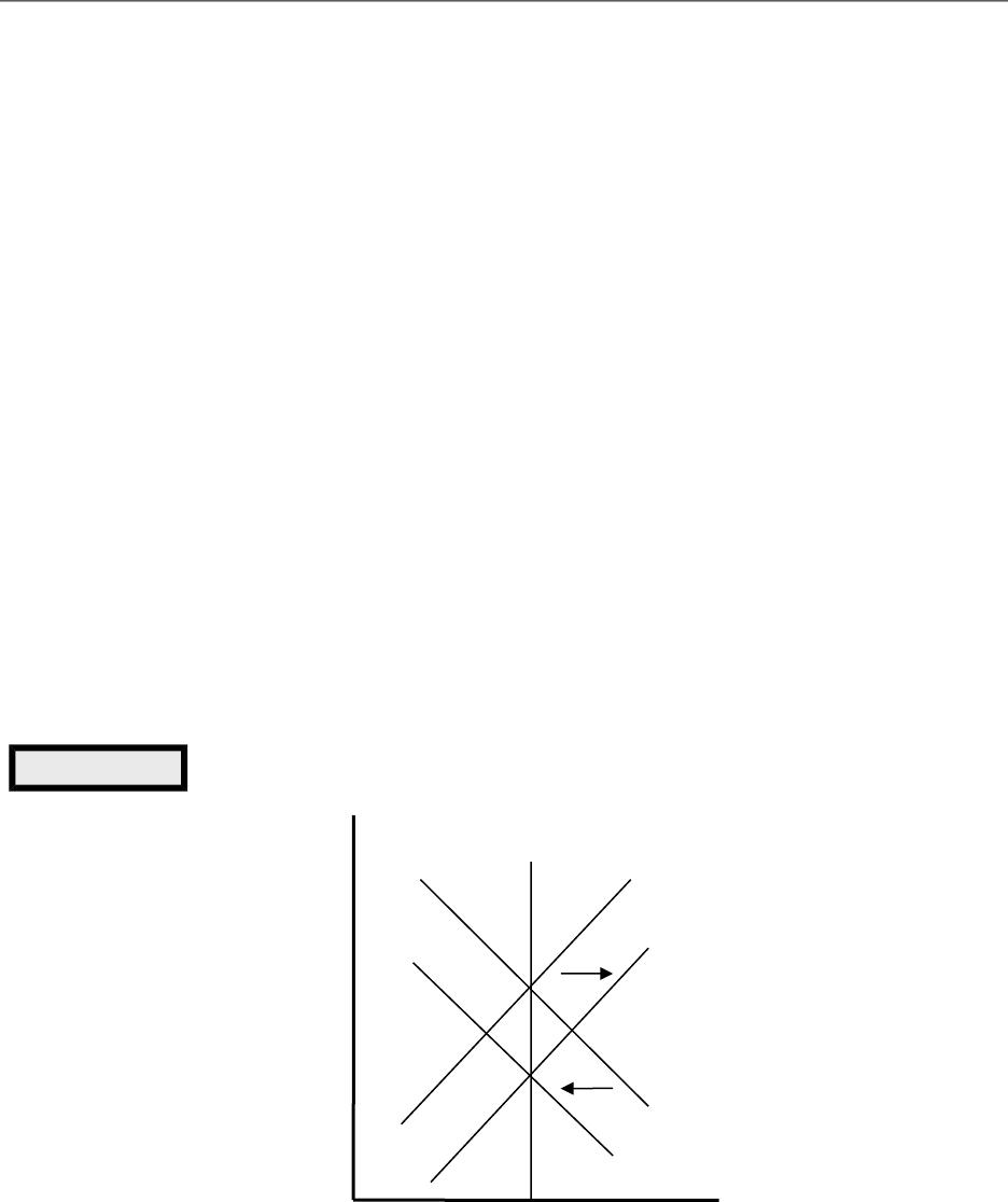
D. Using Aggregate Demand and Aggregate Supply to Depict Long-Run Growth and
In!ation
1. Two important forces that govern the economy in the long run are technological
progress and monetary policy.
a. Technological progress shifts the long-run aggregate-supply curve to the right.
b. The Fed increases the money supply over time, which raises aggregate
demand.
2. The result is growth in output and continuing in!ation (increases in the price
level).
© 2018 Cengage Learning®. May not be scanned, copied or duplicated, or posted to a publicly accessible website,
in whole or in part, except for use as permitted in a license distributed with a certain product or service or otherwise
on a password-protected website or school-approved learning management system for classroom use.
Figure 5
Chapter 33/Aggregate Demand and Aggregate Supply ❖ 555
3. Although the purpose of developing the model of aggregate demand and
aggregate supply is to describe short-run !uctuations, these short-run
!uctuations should be considered deviations from the long-run trends of output
growth and in!ation.
E. Why the Aggregate-Supply Curve Slopes Upward in the Short Run
1. In the short run, the price level does a”ect the economy’s output. An increase in
the overall level of prices tends to raise the quantity of goods and services
supplied.
2. The quantity of output supplied deviates from its natural level when the actual
price level deviates from the expected price level.
3. The Sticky-Wage Theory
a. Nominal wages are often slow to adjust to changing economic conditions due
to long-term contracts between workers and =rms along with social norms and
notions of fairness that in!uence wage setting and are slow to change over
time.
© 2018 Cengage Learning®. May not be scanned, copied or duplicated, or posted to a publicly accessible website,
in whole or in part, except for use as permitted in a license distributed with a certain product or service or otherwise
on a password-protected website or school-approved learning management system for classroom use.
Figure 6

556 ❖ Chapter 33/Aggregate Demand and Aggregate Supply
b. Example: Suppose a =rm has agreed in advance to pay workers an hourly
wage of $20 based on the expectation that the price level will be 100. If the
price level is actually 95, the =rm receives 5% less for its output than it
expected and its labor costs are =xed at $20 per hour.
c. Production is now less pro=table, so the =rm hires fewer workers and reduces
the quantity of output supplied.
d. Nominal wages are based on expected prices and do not adjust immediately
when the actual price level di”ers from what is expected. This makes the
short-run aggregate-supply curve upward sloping.
e. This theory of short-run aggregate supply is emphasized in the text.
4. The Sticky-Price Theory
a. The prices of some goods and services are also sometimes slow to respond to
changing economic conditions. This is often blamed on menu costs.
b. If the price level falls unexpectedly, and a =rm does not change the price of its
product quickly, its relative price will rise and this will lead to a loss in sales.
c. Thus, when sales decline, =rms will produce a lower quantity of goods and
services.
d. Because not all prices adjust instantly to changing conditions, an unexpected
fall in the price level leaves some =rms with higher-than-desired prices, which
depress sales and cause =rms to reduce the quantity of goods and services
supplied.
5. The Misperceptions Theory
© 2018 Cengage Learning®. May not be scanned, copied or duplicated, or posted to a publicly accessible website,
in whole or in part, except for use as permitted in a license distributed with a certain product or service or otherwise
on a password-protected website or school-approved learning management system for classroom use.

Chapter 33/Aggregate Demand and Aggregate Supply ❖ 557
a. Changes in the overall price level can temporarily mislead suppliers about
what is happening in the markets in which they sell their output.
b. As a result of these misperceptions, suppliers respond to changes in the level
of prices and thus, the short-run aggregate-supply curve is upward sloping.
c. Example: The price level falls unexpectedly. Suppliers mistakenly believe that
as the price of their product falls, it is a drop in the relative price of their
product. Suppliers may then believe that the reward of supplying their product
has fallen, and thus they decrease the quantity that they supply. The same
misperception may happen if workers see a decline in their nominal wage
(caused by a fall in the price level).
d. Thus, a lower price level causes misperceptions about relative prices, and
these misperceptions lead suppliers to respond to the lower price level by
decreasing the quantity of goods and services supplied.
6. Note that each of these theories suggests that output deviates from its natural
level when the price level deviates from the price level that people expected.
7. Note also that the e”ects of the change in the price level will be temporary.
Eventually people will adjust their price level expectations and output will return
to its natural level; thus, the aggregate-supply curve will be vertical in the long
run.
8. Because the sticky-wage theory is the simplest of the three theories, it is the one
that is emphasized in the text.
F. Summing Up
1. Economists debate which of these theories is correct and it is possible that each
contains an element of truth.
© 2018 Cengage Learning®. May not be scanned, copied or duplicated, or posted to a publicly accessible website,
in whole or in part, except for use as permitted in a license distributed with a certain product or service or otherwise
on a password-protected website or school-approved learning management system for classroom use.

558 ❖ Chapter 33/Aggregate Demand and Aggregate Supply
2. All three theories suggest that output deviates in the short run from its long-run
level when the actual price level deviates from the expected price level.
3. Each of the three theories emphasizes a problem that is likely to be temporary.
a. Over time, nominal wages will become unstuck, prices will become unstuck,
and misperceptions about relative prices will be corrected.
b. In the long run, it is reasonable to assume that wages and prices are !exible
and that people are not confused about relative prices.
G. Why the Short-Run Aggregate-Supply Curve Might Shift
1. Events that shift the long-run aggregate-supply curve will shift the short-run
aggregate-supply curve as well.
2. However, expectations of the price level will a”ect the position of the short-run
aggregate-supply curve even though it has no e”ect on the long-run
aggregate-supply curve.
3. An increase in the expected price level decreases the quantity of goods and
services supplied and shifts the short-run aggregate-supply curve to the left. A
decrease in the expected price level increases the quantity of goods and services
supplied and shifts the short-run aggregate-supply curve to the right.
VI. Two Causes of Economic Fluctuations
A. Long-Run Equilibrium
© 2018 Cengage Learning®. May not be scanned, copied or duplicated, or posted to a publicly accessible website,
in whole or in part, except for use as permitted in a license distributed with a certain product or service or otherwise
on a password-protected website or school-approved learning management system for classroom use.
Table 2
Figure 7
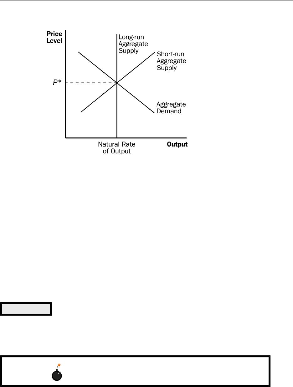
Chapter 33/Aggregate Demand and Aggregate Supply ❖ 559
1. Long-run equilibrium is found where the aggregate-demand curve intersects with
the long-run aggregate-supply curve.
2. Output is at its natural level.
3. Also at this point, perceptions, wages, and prices have all adjusted so that the
short-run aggregate-supply curve intersects at this point as well.
B. The E”ects of a Shift in Aggregate Demand
© 2018 Cengage Learning®. May not be scanned, copied or duplicated, or posted to a publicly accessible website,
in whole or in part, except for use as permitted in a license distributed with a certain product or service or otherwise
on a password-protected website or school-approved learning management system for classroom use.
Table 3
Students will be confused by the graphs showing the adjustment process
that occurs when aggregate demand shifts. Take the time to walk them
through step-by-step several times, summarizing what moves the
560 ❖ Chapter 33/Aggregate Demand and Aggregate Supply
1. Example: Pessimism causes household spending and investment to decline.
2. This will cause the aggregate-demand curve to shift to the left.
3. In the short run, both output and the price level fall. This drop in output means
that the economy is in a recession.
4. In the long run, the economy will move back to the natural rate of output.
a. People will correct the misperceptions, sticky wages, and sticky prices that
cause the aggregate-supply curve to be upward sloping in the short run.
b. The expected price level will fall, shifting the short-run aggregate-supply curve
to the right.
© 2018 Cengage Learning®. May not be scanned, copied or duplicated, or posted to a publicly accessible website,
in whole or in part, except for use as permitted in a license distributed with a certain product or service or otherwise
on a password-protected website or school-approved learning management system for classroom use.
Price
Level
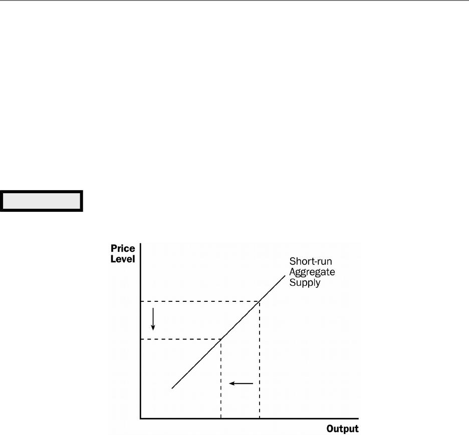
Output
Long-Run Aggregate
Supply
AD1
AD2
AS1
AS2
Figure 8

Chapter 33/Aggregate Demand and Aggregate Supply ❖ 561
5. In the long run, the decrease in aggregate demand can be seen solely by the drop
in the equilibrium price level. Thus, the long-run e”ect of a change in aggregate
demand is a nominal change (in the price level) but not a real change (output is
the same).
6. Instead of waiting for the economy to adjust on its own, policymakers may want
to eliminate the recession by boosting government spending or increasing the
money supply. Either way, these policies could shift the aggregate demand curve
back to the right.
7. FYI: Monetary Neutrality Revisited
a. According to classical theory, changes in the quantity of money a”ect nominal
variables such as the price level, but not real variables such as output.
b. If the Fed decreases the money supply, aggregate demand shifts to the left. In
the short run, output and the price level decline. After expectations, prices,
and wages have adjusted, the economy =nds itself back on the long-run
aggregate-supply curve at the natural level of output.
c. Thus, changes in the money supply have e”ects on real output in the short
run only.
8. Case Study: Two Big Shifts in Aggregate Demand: The Great Depression and
World War II
a. Figure 9 shows real GDP for the United States since 1900.
© 2018 Cengage Learning®. May not be scanned, copied or duplicated, or posted to a publicly accessible website,
in whole or in part, except for use as permitted in a license distributed with a certain product or service or otherwise
on a password-protected website or school-approved learning management system for classroom use.
Figure 9

562 ❖ Chapter 33/Aggregate Demand and Aggregate Supply
b. Two time periods of economic !uctuations can be seen dramatically in the
picture. These are the early 1930s (the Great Depression) and the early 1940s
(World War II).
c. From 1929 to 1933, GDP fell by 27%. From 1939 to 1944, the economy’s
production of goods and services almost doubled.
9. Case Study: The Great Recession of 2008–2009
a. The United States experienced a =nancial crisis and severe economic
downturn in 2008 and 2009.
b. The recession was preceded by a housing boom fueled by low interest rates
and various developments in the mortgage market.
c. From 2006 to 2009, housing values in the U.S. fell by 30%. This led to
substantial defaults, causing additional large losses in the values of
mortgage-backed securities.
d. The economy experienced a large drop in aggregate demand causing real
GDP to fall and unemployment to rise.
10. In the News: Lingering Fears from the Great Recession
a. While the Great Recession oUcially ended in June 2009, Americans have still
not fully recovered.
b. This U.S. News and World Report article explains that Americans have not yet
regained their con=dence in the economy’s long term stability.
© 2018 Cengage Learning®. May not be scanned, copied or duplicated, or posted to a publicly accessible website,
in whole or in part, except for use as permitted in a license distributed with a certain product or service or otherwise
on a password-protected website or school-approved learning management system for classroom use.
Chapter 33/Aggregate Demand and Aggregate Supply ❖ 563
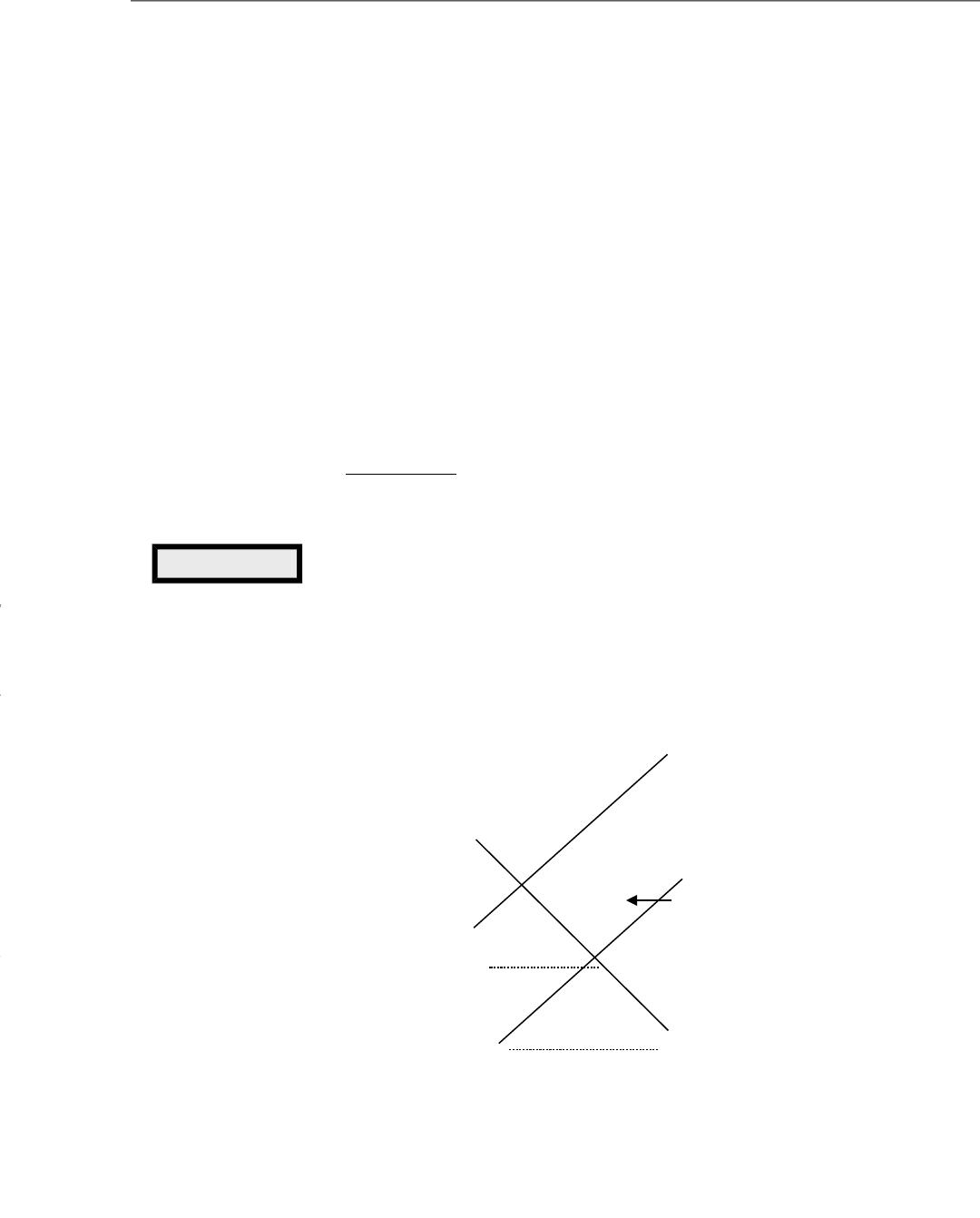
C. The E”ects of a Shift in Aggregate Supply
1. Example: Firms experience a sudden increase in their costs of production.
2. This will cause the short-run aggregate-supply curve to shift to the left.
(Depending on the event, long-run aggregate supply may also shift. We will
assume that it does not.)
3. In the short run, output will fall and the price level will rise. The economy is
experiencing stag!ation.
4. De=nition of stag0ation: a period of falling output and rising prices.
© 2018 Cengage Learning®. May not be scanned, copied or duplicated, or posted to a publicly accessible website,
in whole or in part, except for use as permitted in a license distributed with a certain product or service or otherwise
on a password-protected website or school-approved learning management system for classroom use.
Price
Level
Long-Run
Aggregate Supply
AD
AS2
AS1
P*1
P*2
Figure 10
564 ❖ Chapter 33/Aggregate Demand and Aggregate Supply
5. The result over time may be a wage-price spiral.
6. Eventually, the low level of output will put downward pressure on wages.
a. Producing goods and services becomes more pro=table.
b. Short-run aggregate supply shifts to the right until the economy is again
producing at the natural level of output.
7. If policymakers want to end the stag!ation, they can shift the aggregate-demand
curve. Note that they cannot simultaneously o”set the drop in output and the rise
in the price level. If they increase aggregate demand, the recession will end, but
the price level will be permanently higher.
8. Case Study: Oil and the Economy
a. Crude oil is a key input in the production of many goods and services.
b. When some event (often political) leads to a rise in the price of crude oil, =rms
must endure higher costs of production and the short-run aggregate-supply
curve shifts to the left.
c. In the mid-1970s, OPEC lowered production of oil and the price of crude oil
rose substantially. The in!ation rate in the United States was pushed to over
10%. Unemployment also grew from 4.9% in 1973 to 8.5% in 1975.
© 2018 Cengage Learning®. May not be scanned, copied or duplicated, or posted to a publicly accessible website,
in whole or in part, except for use as permitted in a license distributed with a certain product or service or otherwise
on a password-protected website or school-approved learning management system for classroom use.
Figure 11
Output

Chapter 33/Aggregate Demand and Aggregate Supply ❖ 565
d. This occurred again in the late 1970s. Oil prices rose, output fell, and the rate
of in!ation increased.
e. In the late 1980s, OPEC began to lose control over the oil market as members
began cheating on the agreement. Oil prices fell, which led to a rightward shift
of the short-run aggregate-supply curve. This caused both unemployment and
in!ation to decline.
9. FYI: The Origins of the Model of Aggregate Demand and Aggregate Supply
a. The AD/AS model is a by-product of the Great Depression.
b. In 1936, economist John Maynard Keynes published a book that attempted to
explain short-run !uctuations.
c. Keynes believed that recessions occur because of inadequate demand for
goods and services.
d. Therefore, Keynes advocated policies to increase aggregate demand.
© 2018 Cengage Learning®. May not be scanned, copied or duplicated, or posted to a publicly accessible website,
in whole or in part, except for use as permitted in a license distributed with a certain product or service or otherwise
on a password-protected website or school-approved learning management system for classroom use.

566 ❖ Chapter 33/Aggregate Demand and Aggregate Supply
Activity 1—National Output Article
Type: Take-home assignment
Topics: Fluctuations in output and the price level
Class limitations: Works in any class
Purpose:
This assignment is a good way for students to connect economic theory to actual
events.
Assignment:
1. Find an article in a recent newspaper or magazine illustrating a change that
will a”ect national output.
2. Analyze the situation using economic reasoning.
3. Draw an aggregate demand and aggregate supply graph to explain this
change. Be sure to label your graph and clearly indicate which curve shifts.
Explain what happens to national income and to the price level in the short
run.
© 2018 Cengage Learning®. May not be scanned, copied or duplicated, or posted to a publicly accessible website,
in whole or in part, except for use as permitted in a license distributed with a certain product or service or otherwise
on a password-protected website or school-approved learning management system for classroom use.

Chapter 33/Aggregate Demand and Aggregate Supply ❖ 567
Activity 2—The Economics of War
Type: In-class assignment
Topics: National income, price levels, total spending, resources
Materials needed: None
Time: 20 minutes
Class limitations: Works in any size class
Purpose:
This assignment asks students to examine their beliefs about the e”ect of war on
the economy. It can be used to examine aggregate demand shifts and aggregate
supply shifts. This assignment can generate lively discussion.
Instructions:
Ask the class to answer the following questions. Give them time to write an
© 2018 Cengage Learning®. May not be scanned, copied or duplicated, or posted to a publicly accessible website,
in whole or in part, except for use as permitted in a license distributed with a certain product or service or otherwise
on a password-protected website or school-approved learning management system for classroom use.