43
Chapter 6
6.1
S
γG
γ
ws
=
;
S
)81.9)(73.2(
8.16
=
6.2
S
ρG
ρ
ws
=
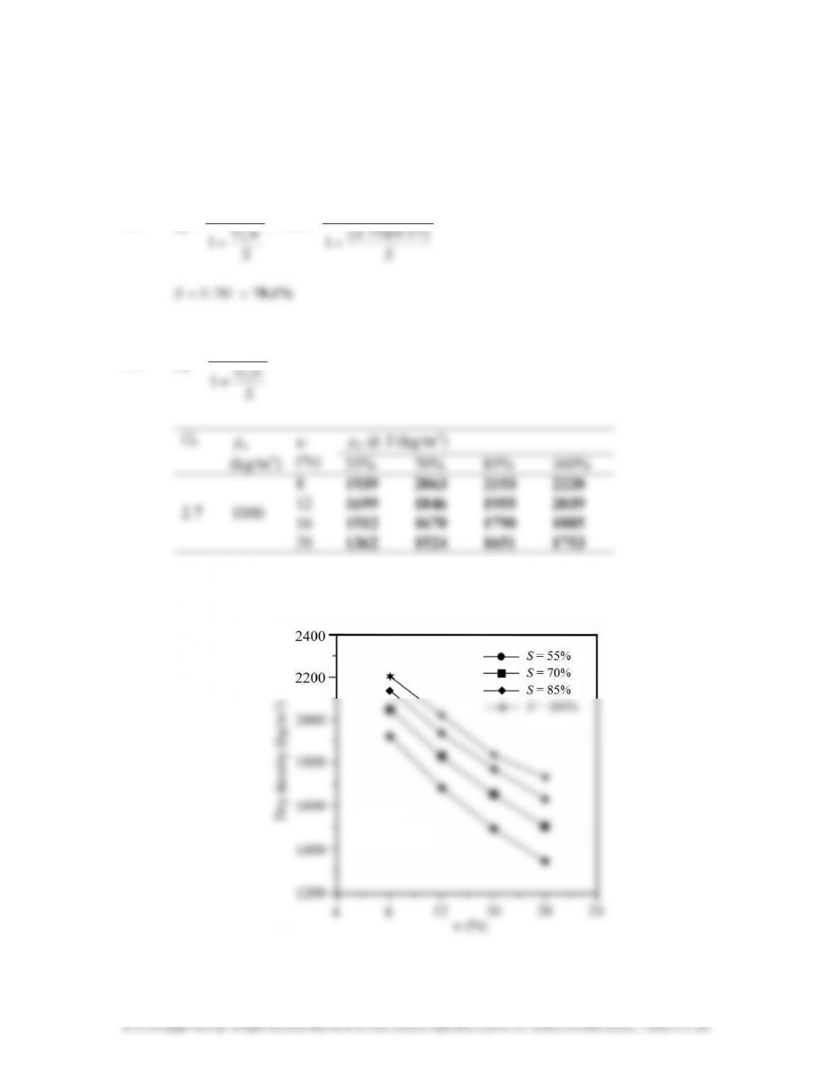
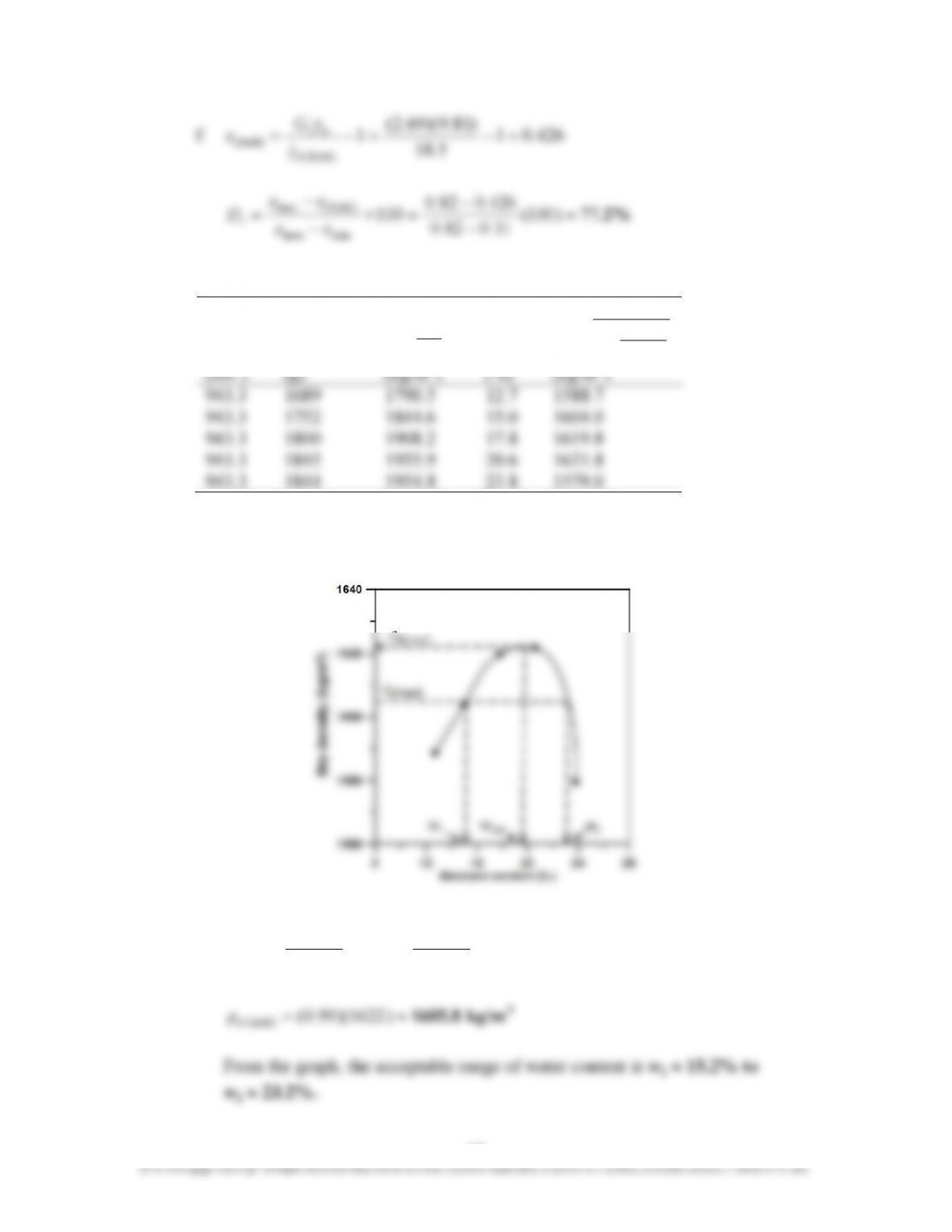
The plot is shown below.
6.3 Eq. (6.4): 376.0
4.62
66.2
4.62
zav
=
=
=
G
γ
γ
w
The table can now be prepared:
w
(%)
)(lb/ft
3
zav
γ
45
© 2018 Cengage Learning®. All Rights Reserved. May not be scanned, copied or duplicated, or posted to a publicly accessible website, in whole or in part.
γG
ws
)4.62)(69.2(
34.0
e
3
124 109.05 lb/ft
γ
6.6
Volume
(ft
3
)
Weight of
soil mass, W
(lb)
V
W
γ=
(lb/ft
3
)
w
(%)
100
(%)
1w
γ
γd+
=
(lb/ft
3
)
1
30
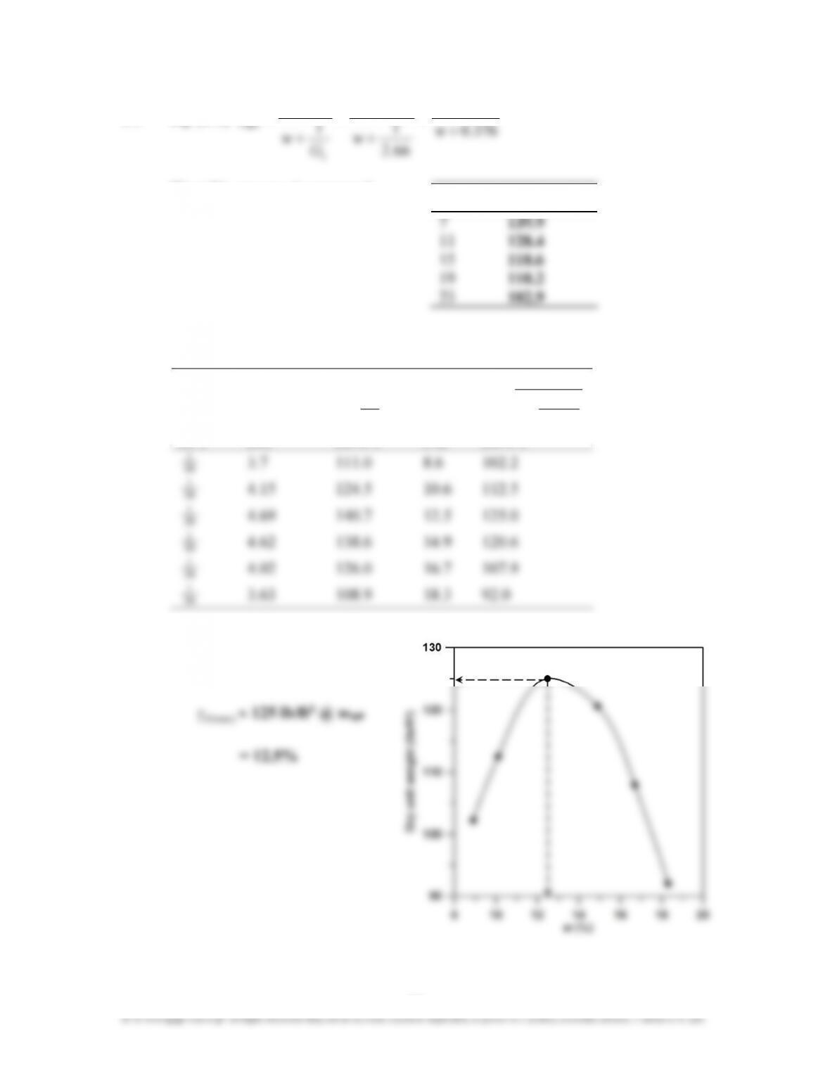
a.
The plot of
d
γvs. w is shown.
(max)d
γ≈ =
3
opt
106.3 lb / ft @ 14.8%w
46
© 2018 Cengage Learning®. All Rights Reserved. May not be scanned, copied or duplicated, or posted to a publicly accessible website, in whole or in part.
b.
6.0;
1
)4.62)(73.2(
3.106;
1≈
+
=
+
=e
ee
γG
γws
d
67.3%==== 673.0
6.0
)73.2)(148.0(
e
wG
Ss
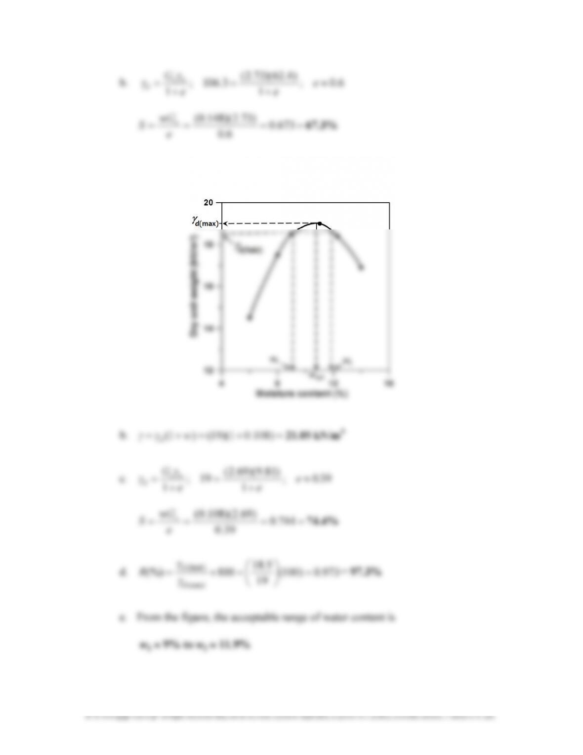
6.7 a. From the figure shown below,
(max)d
γ
≈
19 kN/m
3
@ w
opt
= 10.8%
47
© 2018 Cengage Learning®. All Rights Reserved. May not be scanned, copied or duplicated, or posted to a publicly accessible website, in whole or in part.
f.
426.01
5.18
)81.9)(69.2(
1
)field(
(field)
=−=−=
d
ws
γ
γG
e
77.2%=
−
−
=×
−
−
=)100(
31.082.0
426.082.0
100
minmax
)field(max
ee
ee
D
r
6.8
Volume
3
Mass of
soil, M
V
M
ρ=
3
w
100
(%)
1w
ρ
ρ
d
+
=
3
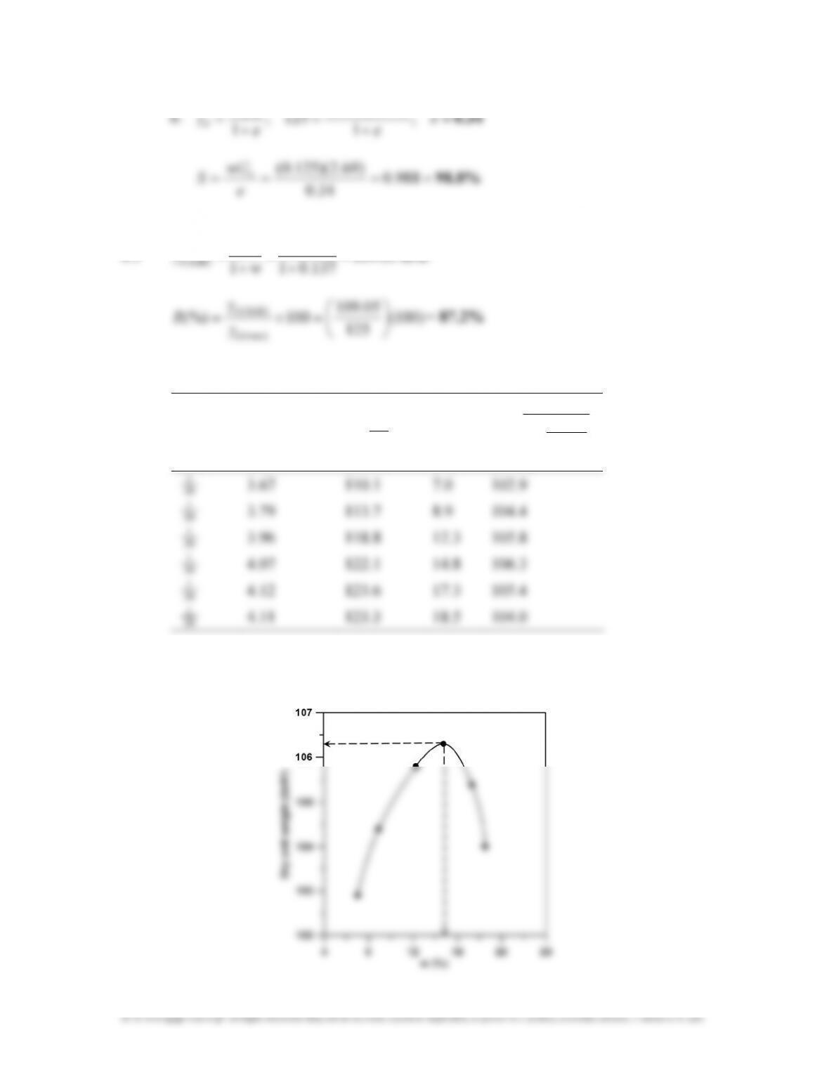
a.
The plot of
d
ρvs. w is shown.
(max)d
ρ
≈
1622 kg/m
3
@ w
opt
≈
19.7%
b.
)100(
1622
100(%)
)field(
(max)
)field(
=×=
d
d
d
ρ
ρ
ρ
R
3
48
6.9 In the field:
+
+
100
1.16
1
100
(%)
1
b. From Problem 6.8:
(max)d
ρ
= 1622 kg/m
3
6.10
3
(in situ)
16.6 kN/m ;
γ=
3
situ) (in
kN/m 95.13
100
19
1
6.16 =
+
=
d
γ;
3
)(compacted
kN/m 5.19=
d
γ
49
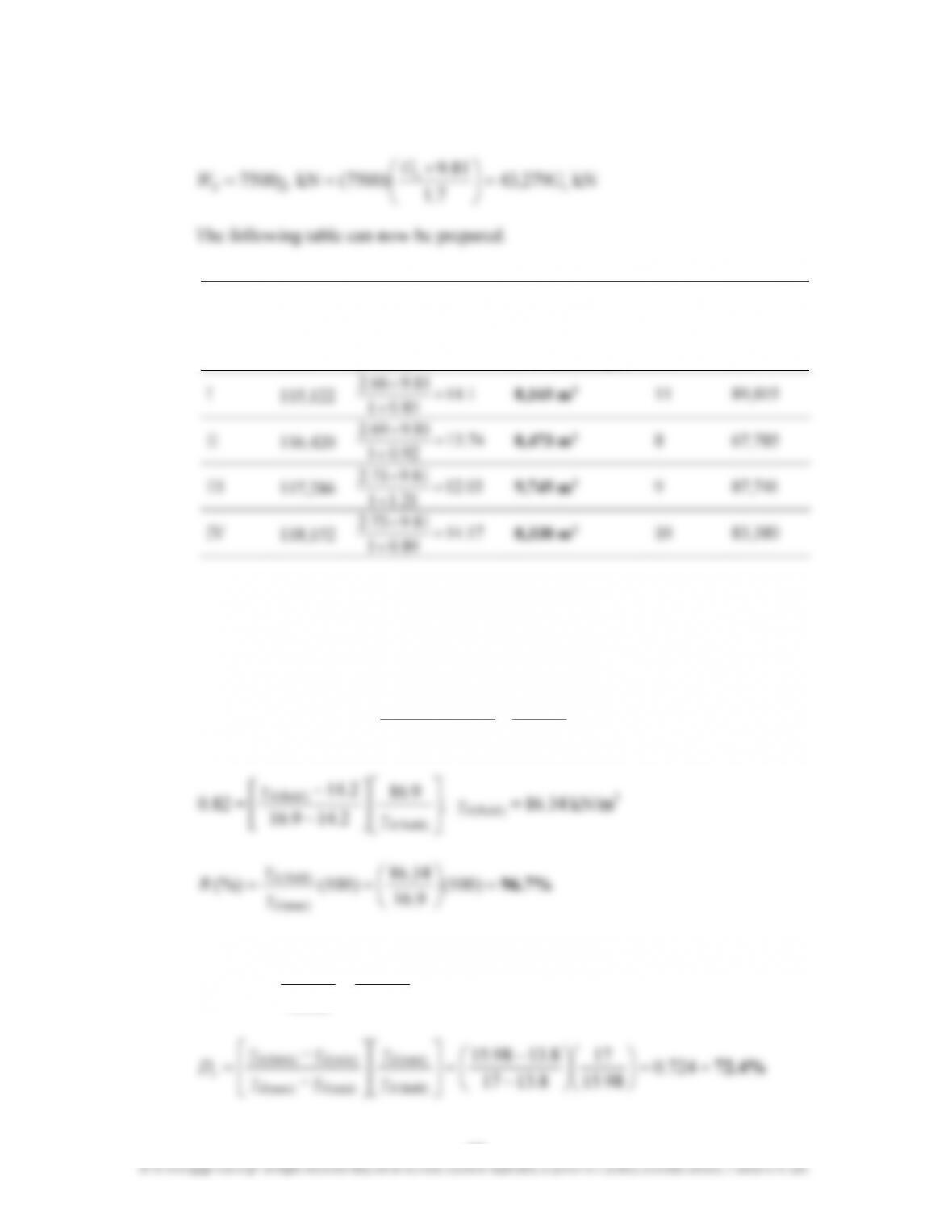
6.11 Dry weight of solids required at the embankment site:
81.9
s
G
×
Borrow
Pit
W
s
(kN)
d
γat borrow pit
(kN/m
3
)
Volume to be
excavated from
borrow pit =
[
)pitborrow (
/
ds γW
]
Cost/m
3
($)
Total
cost
($)
81.966.2 =
×
3
89
.
0
1
+
a.
Shown in table.
b.
Borrow Pit II
6.12 From Eq. (6.22):
−
−
=
)field(
(max)
(min)(max)
(min))field(
d
d
dd
dd
r
γ
γ
γγ
γγ
D
6.13
3
kN/m 15.98====
)field(
)field(
(max)
)field(
;
17
94.0
d
d
d
d
γ
γ
γ
γ
R
−
−
98.15
8.1317
)field(
(min)(max)
d
dd
r
γ
γγ
50
6.14 a.
3
lb/ft 103.5====
)field(
)field(
)field(
;
115
90.0
d
d
d
γ
γ
γ
γ
R
6.15 After compaction:
609.01
5.103
)4.62)(67.2(
1
)field(
(field)
=−=−=
d
ws
γ
γG
e

51
CRITICAL THINKING PROBLEM
6.C.1 a. Osman et al. (2008) method: Eqs. (6.15) through (6.18) are used to calculate
w
opt
and γ
d
(max)
. These values are listed in the table below.
b.
Gurtug and Sridharan (2004) method: Eqs. (6.13) and (6.14) are used to
calculate w
opt
and γ
d
(max)
. These values are listed in the table below.
c.
Matteo et al. (2009) method: Eqs. (6.19) and (6.20) are used to calculate w
opt
and γ
d
(max)
, only for the modified Proctor tests. These values are listed in the
table below.
Soil E
(kN-m/m
3
)
w
opt
(Exp.)
(%)
γ
d(max)
(Exp.)
(kN/m
3
)
Part a Part b Part c
w
opt
(%)
γ
d(max)
(kN/m
3
)
w
opt
(%)
γ
d(max)
(kN/m
3
)
w
opt
(%)
γ
d(max)
(kN/m
3
)
52
© 2018 Cengage Learning®. All Rights Reserved. May not be scanned, copied or duplicated, or posted to a publicly accessible website, in whole or in part.
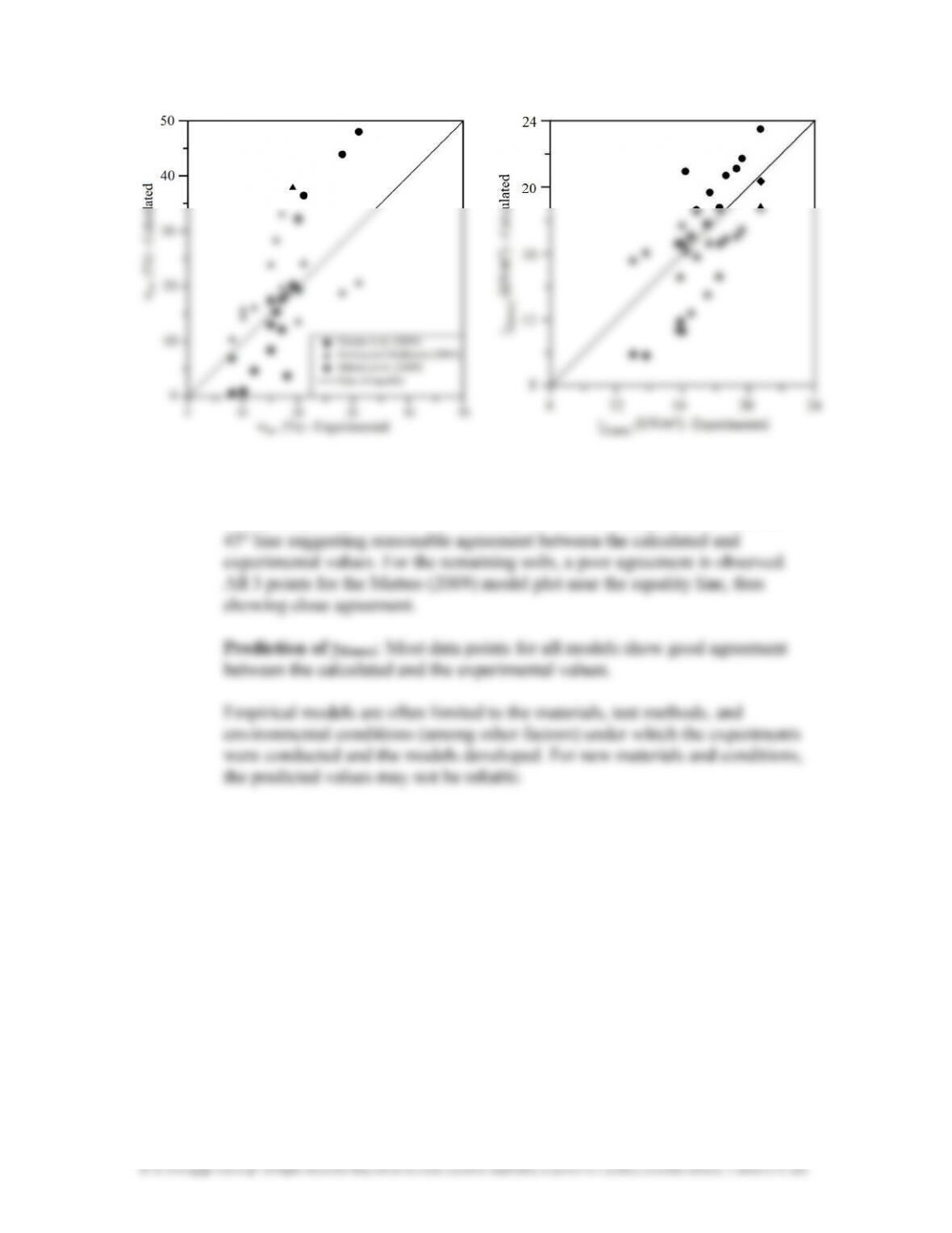
e.
Prediction of
w
opt
: For both the Osman et al. (2008) and Gurtug and
Sridharan (2004) models, several data points are closely packed around the