Unlock document.
This document is partially blurred.
Unlock all pages and 1 million more documents.
Get Access
1
2
3
4
5
6
7
8
9
10
11
12
13
14
15
16
17
18
19
20
21
22
23
24
25
26
27
28
29
30
31
32
33
34
35
36
37
38
39
40
41
42
43
44
46
47
A B C D E F
10/28/2015
Amount invested $1,000
Amount received in one year $1,060
Dollar return (Profit) $60
Rate of return = Profit/Investment = 6%
Worst Case 0.10 −%
Poor Case 0.20 −%
Good Case 0.20 16%
Best Case 0.10 26%
Return on a
10-Year Zero
Coupon
Treasury
Bond During
Next Year
Probability of
Scenario
CHAPTER 6 MINI CASE
a. What are investment returns? What is the return on an investment that costs $1,000 and is sold after 1 year
for $1,060?
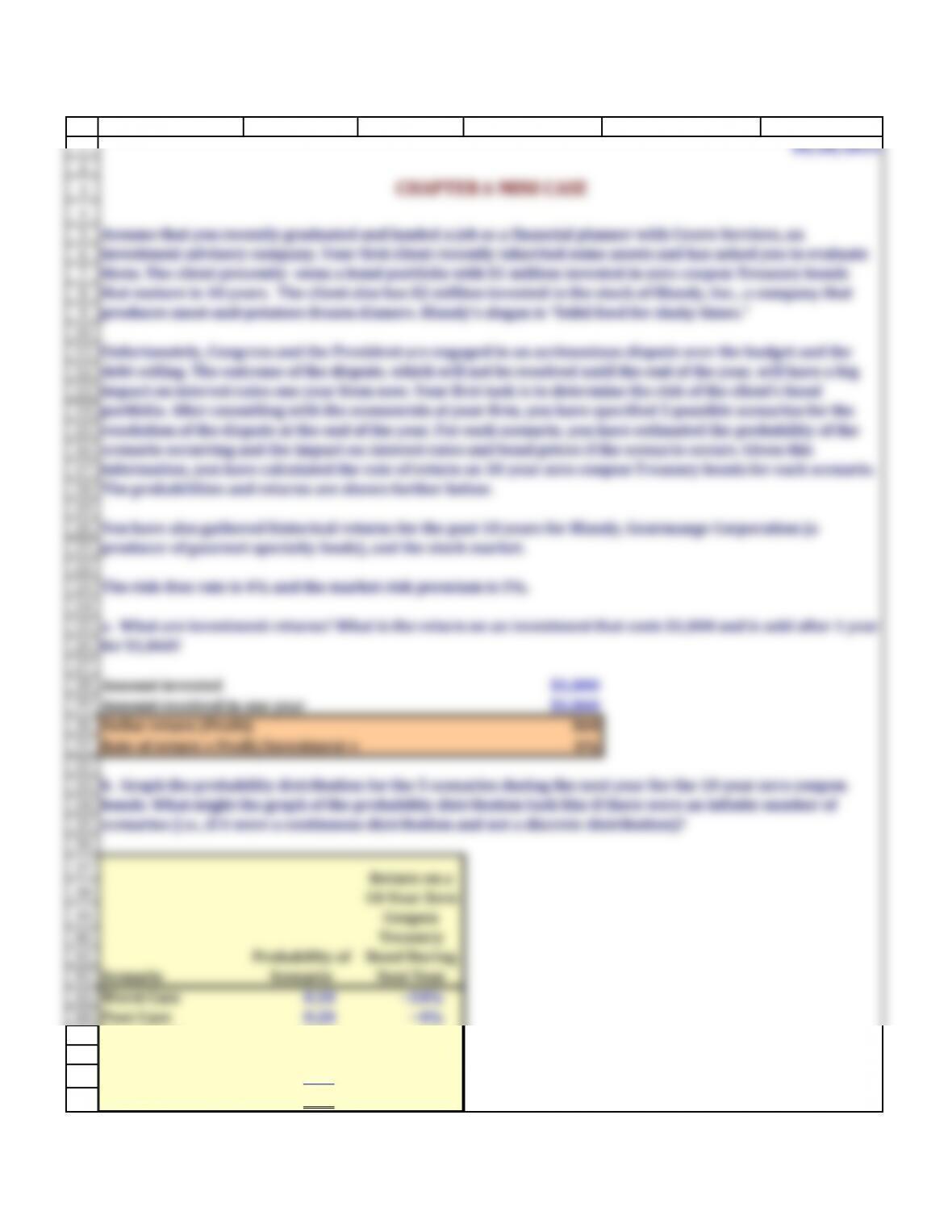
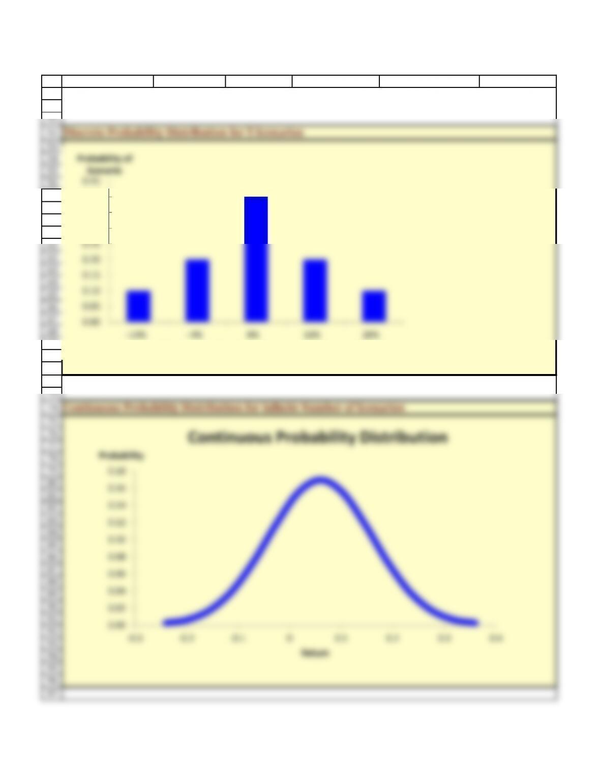
b. Graph the probability distribution for the 5 scenarios during the next year for the 10-year zero coupon
bonds. What might the graph of the probability distribution look like if there were an infinite number of
scenarios (i.e., if it were a continuous distribution and not a discrete distribution)?
You have also gathered historical returns for the past 10 years for Blandy, Gourmange Corporation (a
producer of gourmet specialty foods), and the stock market.
The risk-free rate is 4% and the market risk premium is 5%.
Assume that you recently graduated and landed a job as a financial planner with Cicero Services, an
investment advisory company. Your first client recently inherited some assets and has asked you to evaluate
them. The client presently owns a bond portfolio with $1 million invested in zero coupon Treasury bonds
that mature in 10 years. The client also has $2 million invested in the stock of Blandy, Inc., a company that
produces meat-and-potatoes frozen dinners. Blandy’s slogan is Solid food for shaky times.
Unfortunately, Congress and the President are engaged in an acrimonious dispute over the budget and the
debt ceiling. The outcome of the dispute, which will not be resolved until the end of the year, will have a big
impact on interest rates one year from now. Your first task is to determine the risk of the client’s bond
portfolio. After consulting with the economists at your firm, you have specified 5 possible scenarios for the
resolution of the dispute at the end of the year. For each scenario, you have estimated the probability of the
scenario occurring and the impact on interest rates and bond prices if the scenario occurs. Given this
information, you have calculated the rate of return on 10-year zero coupon Treasury bonds for each scenario.
The probabilities and returns are shown further below.
Scenario
49
50
51
52
53
A B C D E F
Discrete Probability Distribution for 5 Scenarios
98
99
100
101
102
103
104
106
107
108
109
A B C D E F
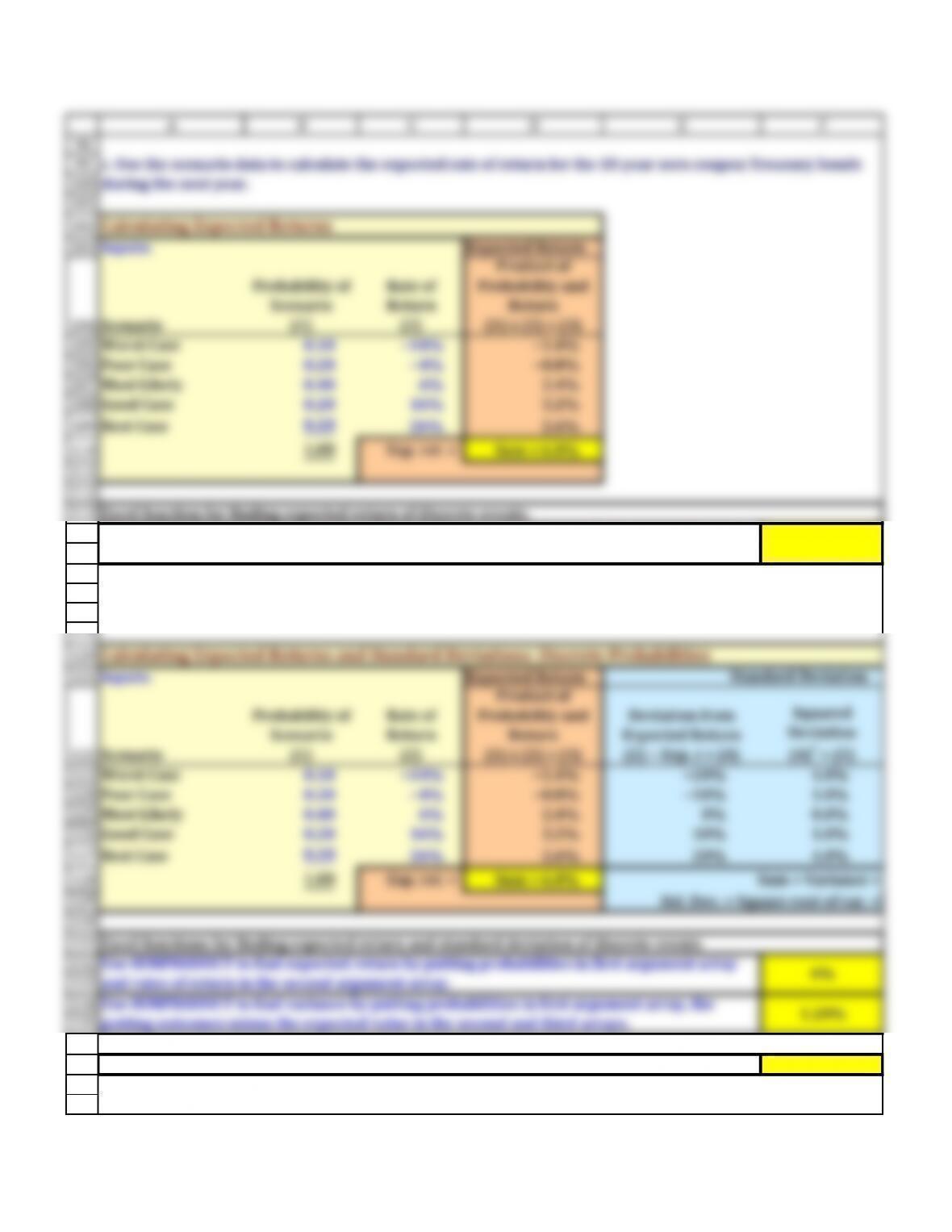
Calculating Expected Returns
Inputs: Expected Return
Scenario
Probability of
Scenario
(1)
Rate of
Return
(2)
Product of
Probability and
Return
(1) x (2) = (3)
Poor Case 0.20 −% −.%
Most Likely 0.40 6% 2.4%
Good Case 0.20 16% 3.2%
Best Case 0.10 26% 2.6%
c. Use the scenario data to calculate the expected rate of return for the 10-year zero coupon Treasury bonds
during the next year.
140
141
142
143
144
145
146
147
148
149
150
151
152
153
159
A B C D E F
Year Market Blandy Gourmange
130% 26% 47%
27% 15% -54%
318% -14% 15%
4 -22% -15% 7%
5 -14% 2% -28%
610% -18% 40%
Standard deviation of returns: 20.1% 25.2% 38.6%
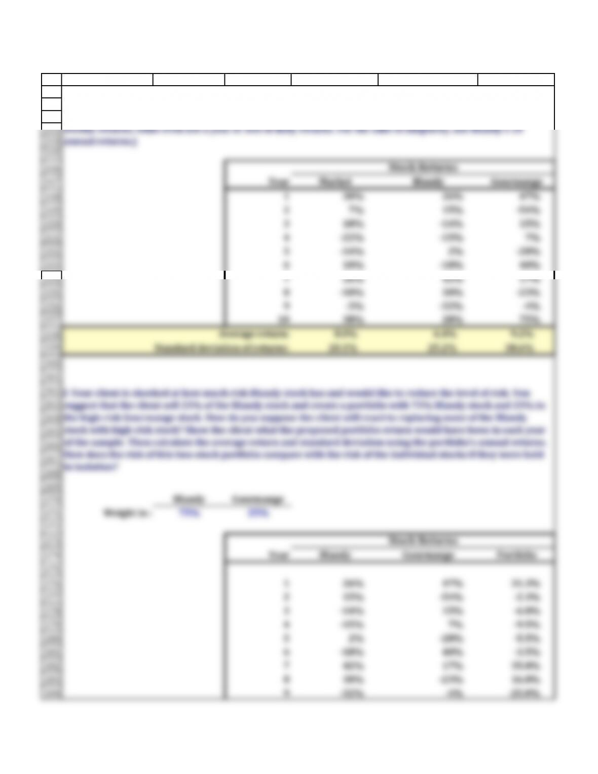
e. Your client has decided that the risk of the bond portfolio is acceptable and wishes to leave it as it is. Now
your client has asked you to use historical returns to estimate the standard deviation of Blandy’s stock
returns. (Note: Many analysts use 4 to 5 years of monthly returns to estimate risk and many use 52 weeks of
weekly returns; some even use a year or less of daily returns. For the sake of simplicity, use Blandy’s
annual returns.)
Stock Returns
185
186
187
188
189
190
191
192
193
194
195
196
202
203
204
205
206
207
213
A B C D E F
10 28% 75% 39.8%
Average return: 6.4% 9.2% 7.1%
Standard deviation of returns: 25.2% 38.6% 22.2%
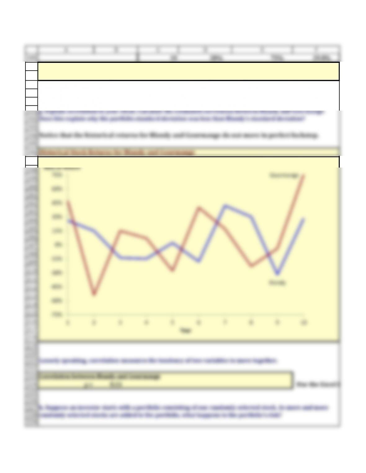
Notice that the historical returns for Blandy and Gourmange do not move in perfect lockstep.
g. Explain correlation to your client. Calculate the estimated correlation between Blandy and Gourmange.
Does this explain why the portfolio standard deviation was less than Blandy’s standard deviation?
Historical Stock Returns for Blandy and Gourmange
-60%
0%
15%
30%
45%
230
231
232
233
234
235
236
237
238
239
240
241
242
243
244
245
246
247
248
249
250
251
252
253
254
255
256
257
258
259
260
261
262
263
264
265
266
267
268
269
270
271
272
273
274
275
276
277
278
A B C D E F
Beta for Stock i = bi = riM(si/sM)
rRF The risk-free rate. It varies over time, but is constant for all firms at a given time.
RPM
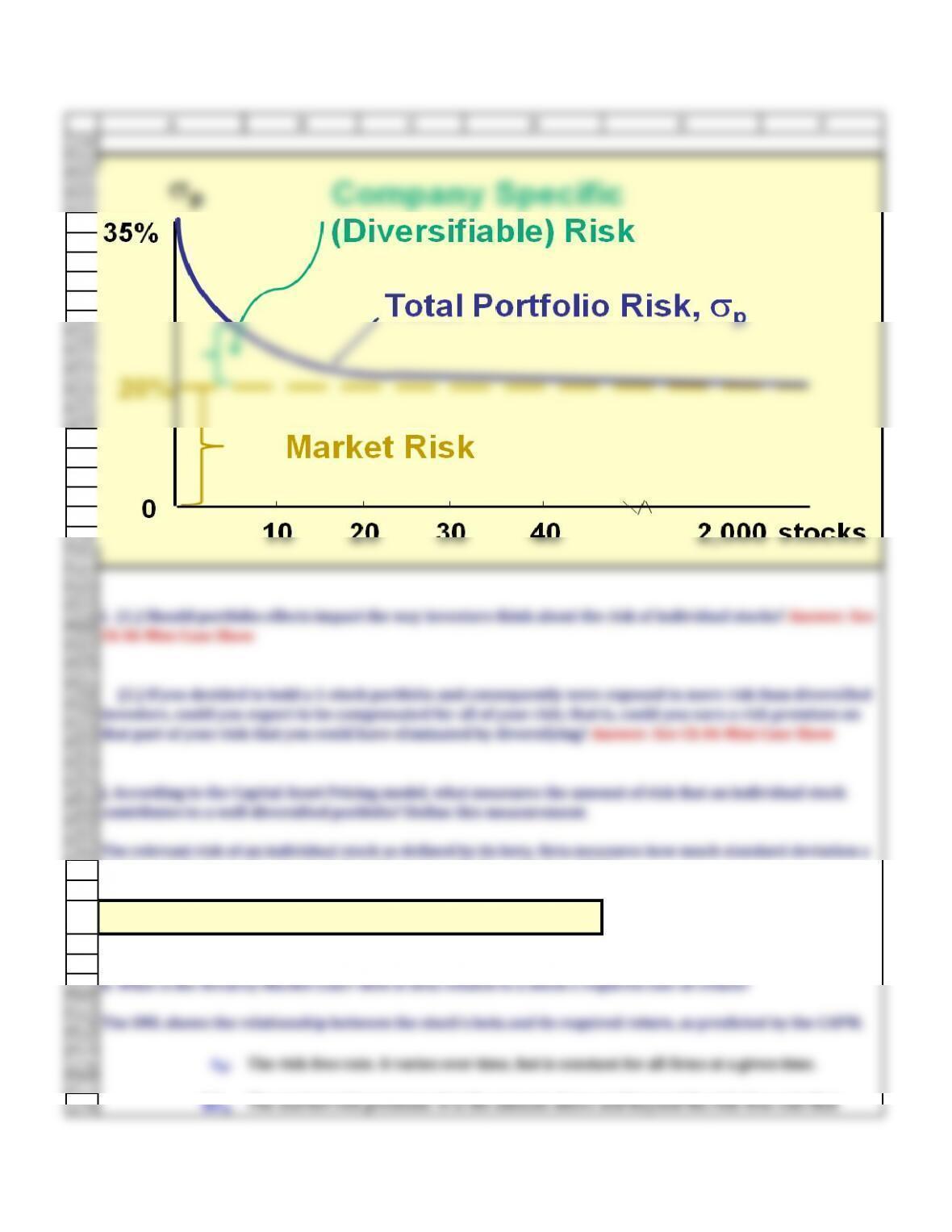
i. (1.) Should portfolio effects impact the way investors think about the risk of individual stocks? Answer: See
Ch 06 Mini Case Show
(2.) If you decided to hold a 1-stock portfolio and consequently were exposed to more risk than diversified
investors, could you expect to be compensated for all of your risk; that is, could you earn a risk premium on
that part of your risk that you could have eliminated by diversifying? Answer: See Ch 06 Mini Case Show
The relevant risk of an individual stock as defined by its beta. Beta measures how much standard deviation a
stock contributes to the standard deviation of a well-diversified portfolio.
k. What is the Security Market Line? (ow is beta related to a stock’s required rate of return?
The SML shows the relationship between the stock's beta and its required return, as predicted by the CAPM.
j. According to the Capital Asset Pricing model, what measures the amount of risk that an individual stock
contributes to a well-diversified portfolio? Define this measurement.
The market risk premium. It is the amount above and beyond the risk-free rate that
investor require to induce them to take on the risk of the stock market. It varies over
time, but is constant for all firms at a given time. Note: the market risk premium can be
279
280
281
282
283
284
285
286
287
288
289
290
291
292
293
295
296
297
298
299
300
301
302
303
311
312
313
314
316
317
319
320
321
322
323
324
325
A B C D E F
biThe beta of stock i. It varies over time, and varies from firm to firm.
ri = rRF + bi (RPM)
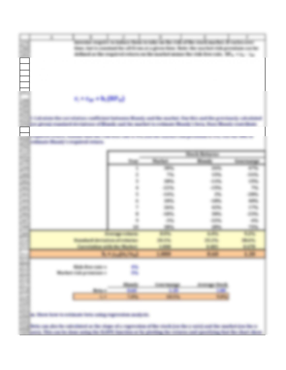
Year Market Blandy Gourmange
130% 26% 47%
27% 15% -54%
318% -14% 15%
4 -22% -15% 7%
5 -14% 2% -28%
Correlation with the Market: 1.000 0.481 0.678
bi = riM(si/sM)1.000 0.60 1.30
Risk-free rate = 4%
Blandy Gourmange Average Stock
ri = 7.0% 10.5% 9.0%
Stock Returns
l. Calculate the correlation coefficient between Blandy and the market. Use this and the previously calculated
or given standard deviations of Blandy and the market to estimate Blandy’s beta. Does Blandy contribute
more or less risk to a well-diversified portfolio than does the average stock? Use the SML to estimate Blandy’s
estimate Blandy’s required return.
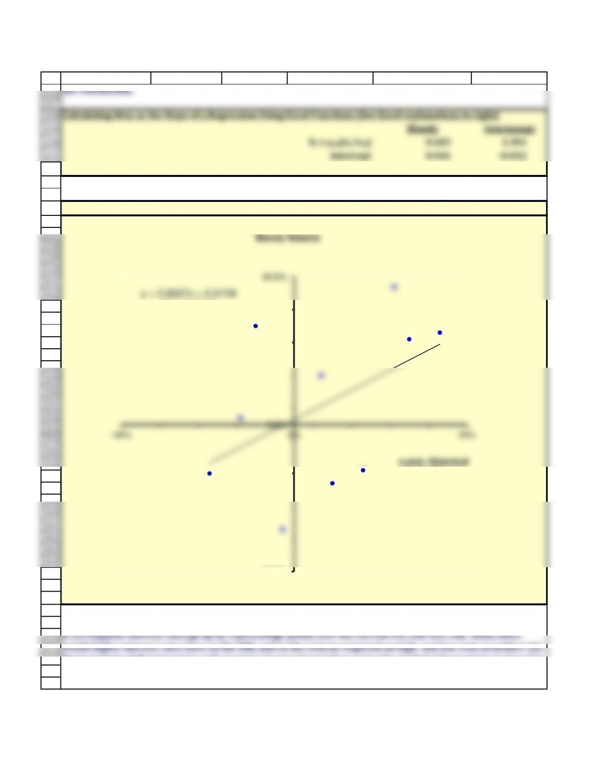
m. Show how to estimate beta using regression analysis.
The SML predicts stock i's required return to be:
Beta can also be calculated as the slope of a regression of the stock (on the y-axis) and the market (on the x-
axis). This can be done using the SLOPE function or by plotting the returns and specifying that the chart show
the TRENDLINE.
The market risk premium. It is the amount above and beyond the risk-free rate that
investor require to induce them to take on the risk of the stock market. It varies over
time, but is constant for all firms at a given time. Note: the market risk premium can be
defined as the required return on the market minus the risk-free rate, RPM = rM - rRF
326
327
328
329
330
331
332
333
334
337
338
339
340
341
342
343
344
345
346
347
348
349
350
351
352
353
354
355
356
357
358
359
360
361
362
363
364
365
370
371
372
373
374
A B C D E F
Blandy Gourmange
bi = riM(si/sM)0.603 1.301
Intercept 0.016 -0.012
R squared 0.232 0.460
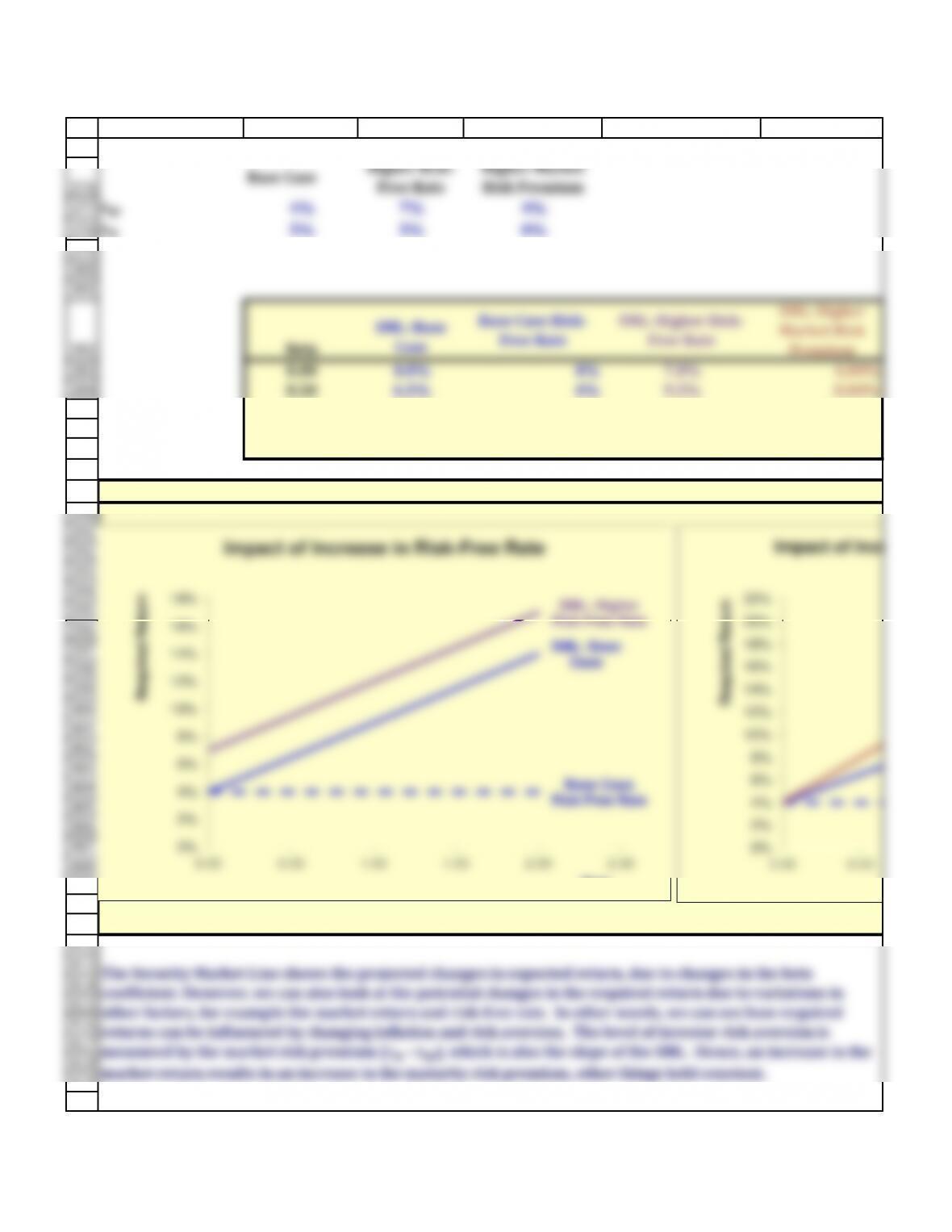
n. (1) Suppose interest rates go up by 3 percentage points over the current 4% risk-free rate. What effect
would higher interest rates have on the SML and on the returns required on high- and low-risk securities? (2)
Suppose instead that investors’ risk aversion increased enough to cause the market risk premium to increase
by 3 percentage points. (Assume the risk-free rate remains constant.) What effect would this have on the SML
and on returns of high- and low-risk securities?
Calculating Beta as the Slope of a Regression Using Excel Functions (See Excel explanations to right)
axis). This can be done using the SLOPE function or by plotting the returns and specifying that the chart show
the TRENDLINE.
y = 0.6027x + 0.0158
R² = 0.2316
-45.0%
0.0%
45.0%
-45% 0% 45%
Blandy Returns
x-axis: Historical
Market Returns
375
376
377
378
379
380
381
382
383
384
385
386
387
389
390
391
392
393
394
395
396
397
398
399
400
401
402
403
404
405
406
407
408
409
410
411
412
A B C D E F
Base Case
Higher Risk-
Free Rate
Higher Market
Risk Premium
rRF 4% 7% 4%
rM5% 5% 8%
Beta
SML: Base
Case
Base Case Risk-
Free Rate
SML: Higher Risk-
Free Rate
SML: Higher
Market Risk
Premium
0.00 4.0% 4% 7.0% 4.00%
0.50 6.5% 4% 9.5% 8.00%
1.00 9.0% 4% 12.0% 12.00%
1.50 11.5% 4% 14.5% 16.00%
2.00 14.0% 4% 17.0% 20.00%
Changes to Inputs for the Security Market Line
SML: Base
Case
Base Case
Risk-Free Rate
SML: Higher
Risk-Free Rate
0%
2%
4%
6%
8%
10%
12%
14%
16%
18%
0.00 0.50 1.00 1.50 2.00 2.50
Required Return
Beta
Impact of Increase in Risk-Free Rate
0%
2%
4%
6%
8%
10%
12%
14%
16%
18%
20%
22%
0.00 0.50
Required Return
Impact of Increase
421
422
423
424
425
426
427
428
429
430
431
433
435
436
437
438
439
442
443
444
445
447
448
449
450
451
452
453
455
457
458
459
460
461
462
463
464
465
A B C D E F
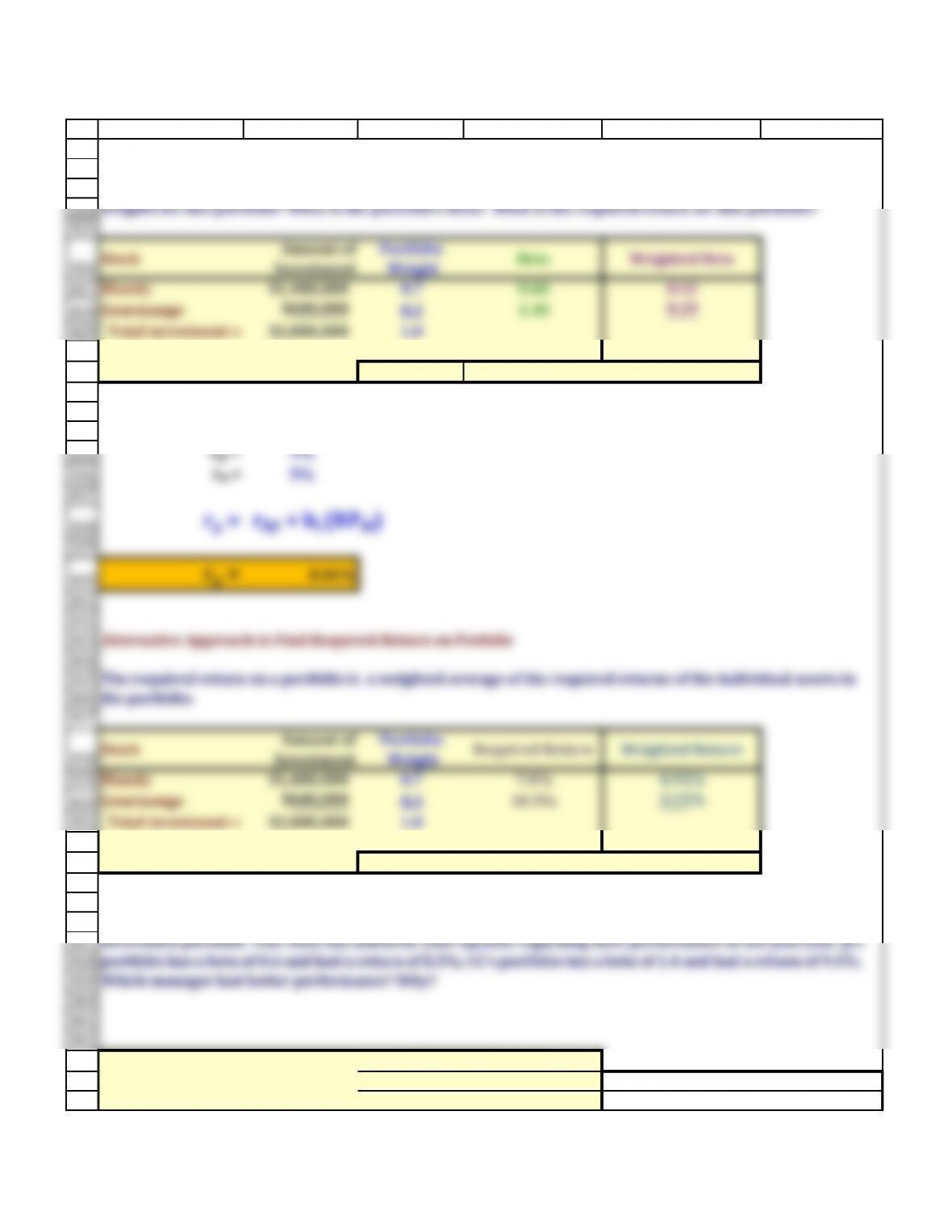
Stock
Amount of
Investment
Portfolio
Weight
Beta Weighted Beta
Blandy $1,400,000 0.7 0.60 0.42
Gourmange $600,000 0.3 1.30 0.39
Total investment = $2,000,000 1.0
Portfolio's Beta = 0.81
rRF = 4%
rM = 5%
rp = rRF + bi (RPM)
Alternative Approach to Find Required Return on Porfolio
Stock
Amount of
Investment
Portfolio
Weight
Required Return Weighted Return
Blandy $1,400,000 0.7 7.0% 4.91%
Gourmange $600,000 0.3 10.5% 3.15%
Total investment = $2,000,000 1.0
Portfolio's Return = 8.06%
JJ CC
Portfolio beta = 0.7 1.4 0 2
o. Your client decides to invest $1.4 million in Blandy stock and $0.6 million in Gourmange stock. What are the
weights for this portfolio? What is the portfolio’s beta? What is the required return for this portfolio?
The required return on a portfolio is a weighted average of the required returns of the individual assets in
Portfolio Manager
Additonal data for graph
diversified portfolio. Your boss has asked for your opinion regarding their performance in the past year. JJ’s
portfolio has a beta of . and had a return of .%; CC’s portfolio has a beta of . and had a return of .%.
Which manager had better performance? Why?


