Unlock document.
This document is partially blurred.
Unlock all pages and 1 million more documents.
Get Access
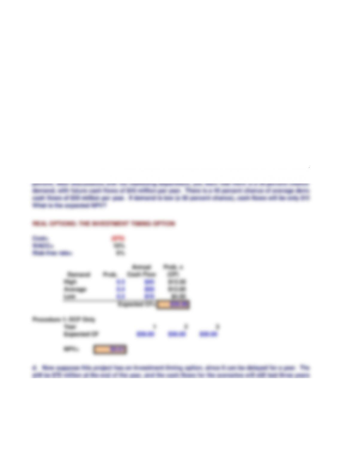
REAL OPTIONS: THE INVESTMENT TIMING OPTION
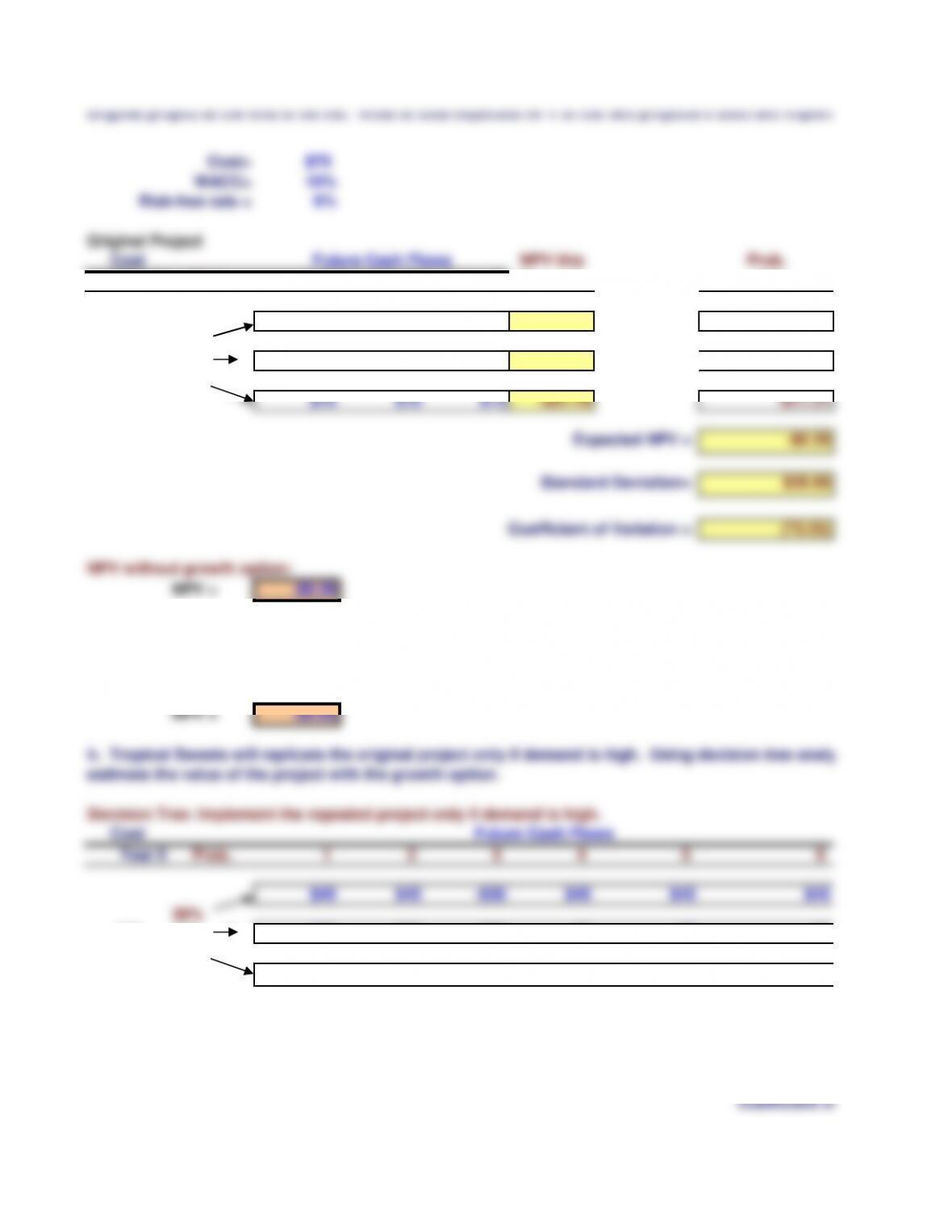
Cost= ($70)
WACC= 10%
Risk-free rate= 6%
Demand Prob.
Annual
Cash Flow
Prob. x
(CF)
High 0.3 $45 $13.50
Average 0.4 $30 $12.00
Low 0.3 $15 $4.50
Expected CF= $30.00
Procedure 1: DCF Only
Year 1 2 3
Expected CF $30.00 $30.00 $30.00
NPV= $4.61
Assume that you have just been hired as a financial analyst by Tropical Sweets Inc., a mid-sized Califo
company that specializes in creating exotic candies from tropical fruits such as mangoes, papayas, an
The firm's CEO, George Yamaguchi, recently returned from an industry corporate executive conference i
Francisco, and one of the sessions he attended was on real options. Since no one at Tropical Sweets i
with the basics of real options, Yamaguchi has asked you to prepare a brief report that the firm's exec
could use to gain at least a cursory understanding of the topics.
a. What are some types of real options? Answer: See Chapter 26 Mini Case Show
b. What are the five steps for analyzing a real option? Answer: See Chapter 26 Mini Case Show
c. Tropical Sweets is considering a project that will cost $70 million and will generate expected cash f
per year for three years. The cost of capital for this type of project is 10 percent and the risk-free rate is
percent. After discussions with the marketing department, you learn that there is a 30 percent chance of
demand, with future cash flows of $45 million per year. There is a 40 percent chance of average demand
cash flows of $30 million per year. If demand is low (a 30 percent chance), cash flows will be only $15 per
What is the expected NPV?
d. Now suppose this project has an investment timing option, since it can be delayed for a year. The c
still be $70 million at the end of the year, and the cash flows for the scenarios will still last three years.
Tropical Sweets will know the level of demand, and will implement the project only if it adds value to th
company. Perform a qualitative assessment of the investment timing option’s value. Answer: See Ch
Mini Case Show
Chapter 26. Real Options
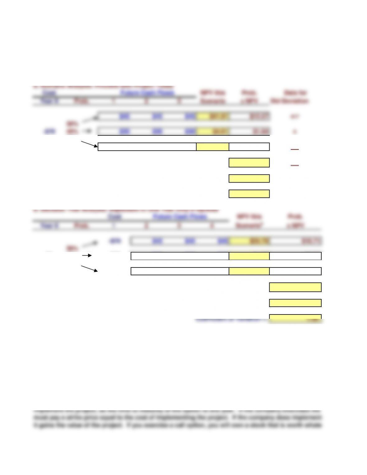
Procedure 3: Decision Tree Analysis
a. Scenario Analysis: Proceed with Project Today
Cost NPV this Prob. Data for
Year 0 Prob. 1 2 3 Scenario x NPV
$45 $45 $45 $41.91 $12.57 417
30%
Standard Deviation= $28.89
Coefficient of Variation = 6.27
b. Decision Tree Analysis: Implement in One Year Only if Optimal
Cost NPV this Prob.
Year 0 Prob. 12 3 4
Scenarioax NPV
-$70 $45 $45 $45 $35.70 $10.71
30%
Standard Deviation= $15.91
Coefficient of Variation = 1.39
Notes:
e. Use decision tree analysis to calculate the NPV of the project with the investment timing option.
Std Deviation
Future Cash Flows
Future Cash Flows
a Discount the cost of the project at the risk-free rate, since the cost is known. Discount
the operating cash flows at the WACC.
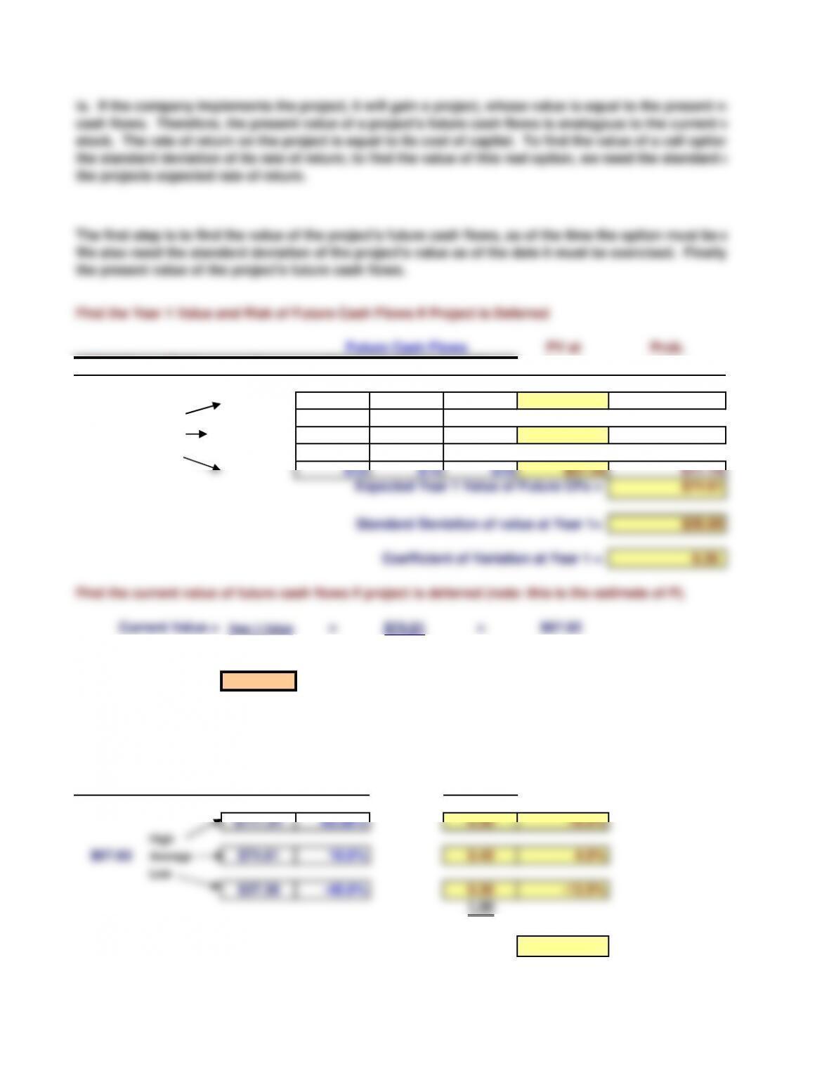
Find the Year 1 Value and Risk of Future Cash Flows If Project is Deferred
PV at Prob.
Year 0 Prob. 1 2 3 4 Year 1 x Value
$45 $45 $45 $111.91 $33.57
Future Cash Flows
is. If the company implements the project, it will gain a project, whose value is equal to the present value of
cash flows. Therefore, the present value of a project's future cash flows is analogous to the current value of
stock. The rate of return on the project is equal to its cost of capital. To find the value of a call option
the standard deviation of its rate of return; to find the value of this real option, we need the standard dev
the projects expected rate of return.
The first step is to find the value of the project's future cash flows, as of the time the option must be e
We also need the standard deviation of the project's value as of the date it must be exercised. Finally, w
the present value of the project's future cash flows.
Standard deviation of return = 42.6%
Direct estimate of s2 = Variance of return = 0.182
CV =Coefficient of Variation = 0.39
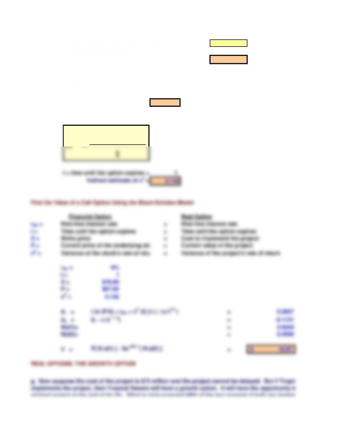
Now use the following formula to estimate the variance of the project's rate of return.
t = time until the option expires = 1
Indirect estimate of s2 = 0.142
Find the Value of a Call Option Using the Black-Scholes Model
Real Option
rRF = Risk-free interest rate = Risk-free interest rate
t = Time until the option expires = Time until the option expires
X = Strike price = Cost to implement the project
P =
Current price of the underlying sto
= Current value of the project
s2 =
Variance of the stock's rate of retur
= Variance of the project's rate of return
rRF = 6%
t = 1
X = $70.00
P = $67.82
Financial Option
Use the indirect approach to estimate the variance of the project's rate of return. Start by estimating th
variation, CV, of the project's value at the time the option expires. This was done in an earlier step.
t
]1CVln[ 2
2+
=s
Cost= $75
WACC= 10%
Risk-free rate = 6%
Original Project
Cost NPV this Prob.
Future Cash Flows
original project at the end of its life. What is total expected NPV of the two projects if both are implement

Notes: 1. The CF in Year 3 includes the cost to implement the second project if it is optimal to do so.
Financial Option Approach
Find the value and risk of the future cash flows as of the time the option expires.
Cost
Year 0 Prob. 1 2 3 4 5 6
$45 $45 $45
30%
40% $30 $30 $30
30%
$15 $15 $15
Find the current value of future cash flows if project is deferred (note: this is the estimate of P).
Current Value = Year 3 Value =$74.61 =$56.05
(1+WACC)3
1.33
P = $56.05
Use the direct approach to estimate the variance of the project's rate of return.
Expected return = 7.968%
Standard deviation of return = 15.0%
i. Use a financial option model to estimate the value of the growth option.
2. When finding the NPV, the cost to implement the second project is discounted at the risk
flows are discounted at the cost of capital.
Future Cash Flows

Direct estimate of s2 = Variance of return = 0.023
CV =Coefficient of Variation = 0.39
Now use the following formula to estimate the variance of the project's rate of return.
t = time until the option expires = 3
Indirect estimate of s2 = 0.047
Find the Value of a Call Option Using the Black-Scholes Model
Sensitivity Analysis
Base Case Case 1
rRF = 6% 6%
t = 3 3
X = $75.00 $75.00
P = $56.05 $56.05
s2 = 0.047 0.142
d1 = =-0.1085 0.1559
d2 = d1 - s (t 1 / 2) = -0.4840 -0.4968
N(d1)= = 0.4568 0.5619
N(d2)= = 0.3142 0.3097
V =
P[ N (d1) ] - Xe-rRF t [ N (d2) ] =5.92$ 12.10$
Total Value = Value of Project 1 + Value of growth option
Total Value = -$0.39 + $5.92
Total Value = 5.53$
{ ln (P/X) + [rRF + s2 /2) ] t }
(s t1/2 )
j. What happens to the value of the growth option if the variance of the project’s return is 14.2 percent? What if it
is 50 percent? How might this explain the high valuations of many dot.com companies?
Use the indirect approach to estimate the variance of the project's rate of return. Start by estimating th
variation, CV, of the project's value at the time the option expires. This was done in an earlier step.
t
]1CVln[ 2
2+
=s


