Unlock document.
This document is partially blurred.
Unlock all pages and 1 million more documents.
Get Access
Chapter 11 Mini Case
Situation
Part I: Input Data
Equipment cost $200,000 Key Output: NPV = $88,010
Shipping charge $10,000
Installation charge $30,000
Economic Life 4
Salvage Value $25,000
Tax Rate 40%
Cost of Capital 10%
Units Sold 1,250
Sales Price Per Unit $200
Incremental Cost Per Unit $100
NWC/Sales 12%
Inflation rate 3%
Shrieves Casting Company is considering adding a new line to its product mix, and the capital budg
analysis is being conducted by Sidney Johnson, a recently graduated MBA. The production line wou
up in unused space in Shrieves' main plant. The machinery’s invoice price would be approximately $200,000,
another $10,000 in shipping charges would be required, and it would cost an additional $30,000 to inst
equipment. The machinery has an economic life of 4 years, and Shrieves has obtained a special tax r
places the equipment in the MACRS 3-year class. The machinery is expected to have a salvage value of
$25,000 after 4 years of use.
The new line would generate incremental sales of 1,250 units per year for 4 years at an incremental cost
$100 per unit in the first year, excluding depreciation. Each unit can be sold for $200 in the first year. T
price and cost are both expected to increase by 3% per year due to inflation. Further, to handle the new
the firm’s net working capital would have to increase by an amount equal to 12% of sales revenues. The firm’s
tax rate is 40%, and its overall weighted average cost of capital, which is the risk-adjusted cost of ca
an average project (r), is 10%.
a. Define “incremental cash flow.” Answer: See Chapter 11 Mini Case Show
(2.) Suppose the firm had spent $100,000 last year to rehabilitate the production line site. Should t
included in the analysis? Explain. Answer: See Chapter 11 Mini Case Show
(1.) Should you subtract interest expense or dividends when calculating project cash flow? Answ
Chapter 11 Mini Case Show
(3.) Now assume that the plant space could be leased out to another firm at $25,000 per year. Sh
be included in the analysis? If so, how? Answer: See Chapter 11 Mini Case Show
(4.) Finally, assume that the new product line is expected to decrease sales of the firm’s other lines by
$50,000 per year. Should this be considered in the analysis? If so, how? Answer: See Chapter 11
Case Show
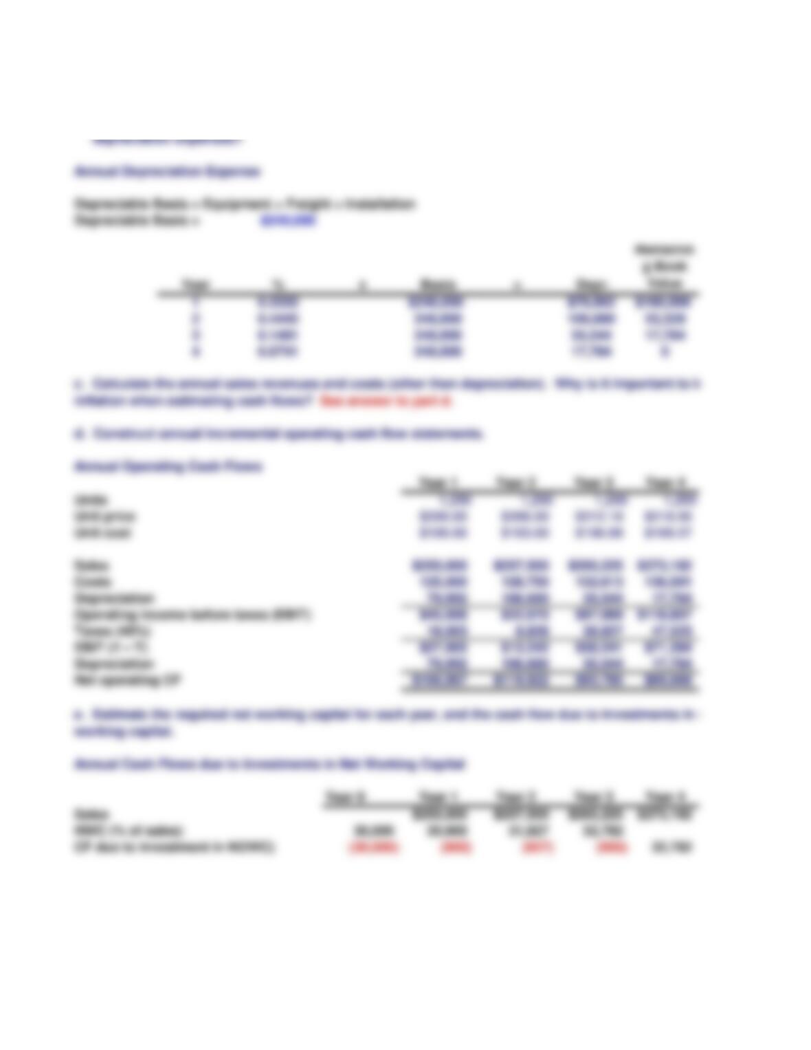
Annual Depreciation Expense
Depreciable Basis = Equipment + Freight + Installation
Depreciable Basis = $240,000
Year % x Basis = Depr.
Remainin
g Book
Value
10.3333 $240,000 $79,992 $160,008
20.4445 240,000 106,680 53,328
30.1481 240,000 35,544 17,784
40.0741 240,000 17,784 0
d. Construct annual incremental operating cash flow statements.
b. Disregard the assumptions in Part a. What is Shrieves' depreciable basis? What are the annual
depreciation expenses?
c. Calculate the annual sales revenues and costs (other than depreciation). Why is it important to includ
inflation when estimating cash flows? See answer to part d.
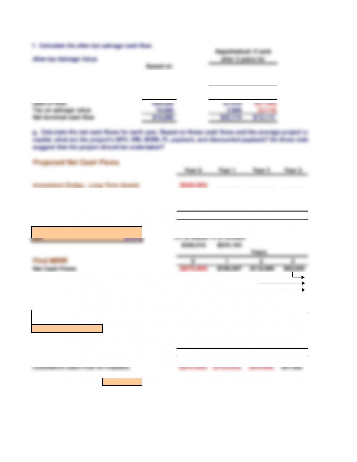
f. Calculate the after-tax salvage cash flow.
After-tax Salvage Value
Based on
facts in
case:
$25,000 $10,000
Salvage value $25,000 $25,000 $10,000
Book value 017,784 17,784
Gain or loss $25,000 $7,216 ($7,784)
Tax on salvage value 10,000 2,886 (3,114)
Net terminal cash flow $15,000 $22,114 $13,114
Projected Net Cash Flows
Year 0 Year 1 Year 2 Year 3
Investment Outlay: Long Term Assets ($240,000)
Operating Cash Flows $106,997 $119,922 $93,785
CF due to investment in NWC (30,000) (900) (927) (955)
Salvage Cash Flows
Net Cash Flows ($270,000) $106,097 $118,995 $92,830
Hypothetical: If sold
after 3 years for
g. Calculate the net cash flows for each year. Based on these cash flows and the average project co
capital, what are the project’s NPV, IRR, MIRR, PI, payback, and discounted payback? Do these indicators
suggest that the project should be undertaken?
% Deviation % Deviation
% Deviation
from Base r NPV from Base units NPV from
Base Salv.
Base Case 10.0% $88,010 Base Case 1,250 $88,010 Base Case $25,000
-30% 7.0% $113,270 -30% 875 $16,649 -30% $17,500
-15% 8.5% $100,291 -15% 1,063 $52,329 -15% $21,250
0% 10.0% $88,010 0% 1,250 $88,010 0% $25,000
15% 11.5% $76,378 15% 1,438 $123,690 15% $28,750
30% 13.0% $65,350 30% 1,625 $159,371 30% $32,500
i. (1.) What are the three types of risk that are relevant in capital budgeting? Answer: See Chapter
Case Show
(3.) How is each type of risk used in the capital budgeting process? Answer: See Chapter 11 Mini Case
Show
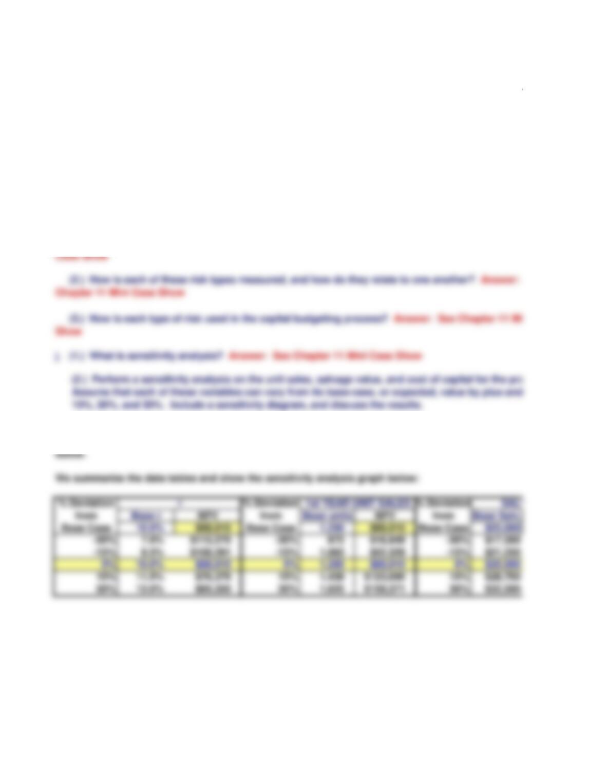
(2.) Perform a sensitivity analysis on the unit sales, salvage value, and cost of capital for the projec
Assume that each of these variables can vary from its base-case, or expected, value by plus and min
10%, 20%, and 30%. Include a sensitivity diagram, and discuss the results.
(2.) How is each of these risk types measured, and how do they relate to one another? Answer:
Chapter 11 Mini Case Show
h. What does the term ”risk” mean in the context of capital budgeting; to what extent can risk be quantified;
and when risk is quantified, is the quantification based primarily on statistical analysis of historical dat
subjective, judgmental estimates?
j. (1.) What is sensitivity analysis? Answer: See Chapter 11 Mini Case Show
Risk in capital budgeting really means the probability that the actual outcome will be worse than the e
outcome. For example, if there were a high probability that the expected NPV as calculated above w
turn out to be negative, then the project would be classified as relatively risky. The reason for a wor
expected outcome is, typically, because sales were lower than expected, costs were higher than expected
and/or the project turned out to have a higher than expected initial cost. In other words, if the assumed
turn out to be worse than expected then the output will likewise be worse than expected. We use Exc
examine the project's sensitivity to changes in the input variables.
r
Here we use an Excel "Data Table" to find the NPVs for changes in unit sales, salvage value, and WA
holding other things constant--changing one variable at a time. This produces the sensitivity analys a
below.
We summarize the data tables and show the sensitivity analysis graph below:
1st YEAR UNIT SALES
SALV
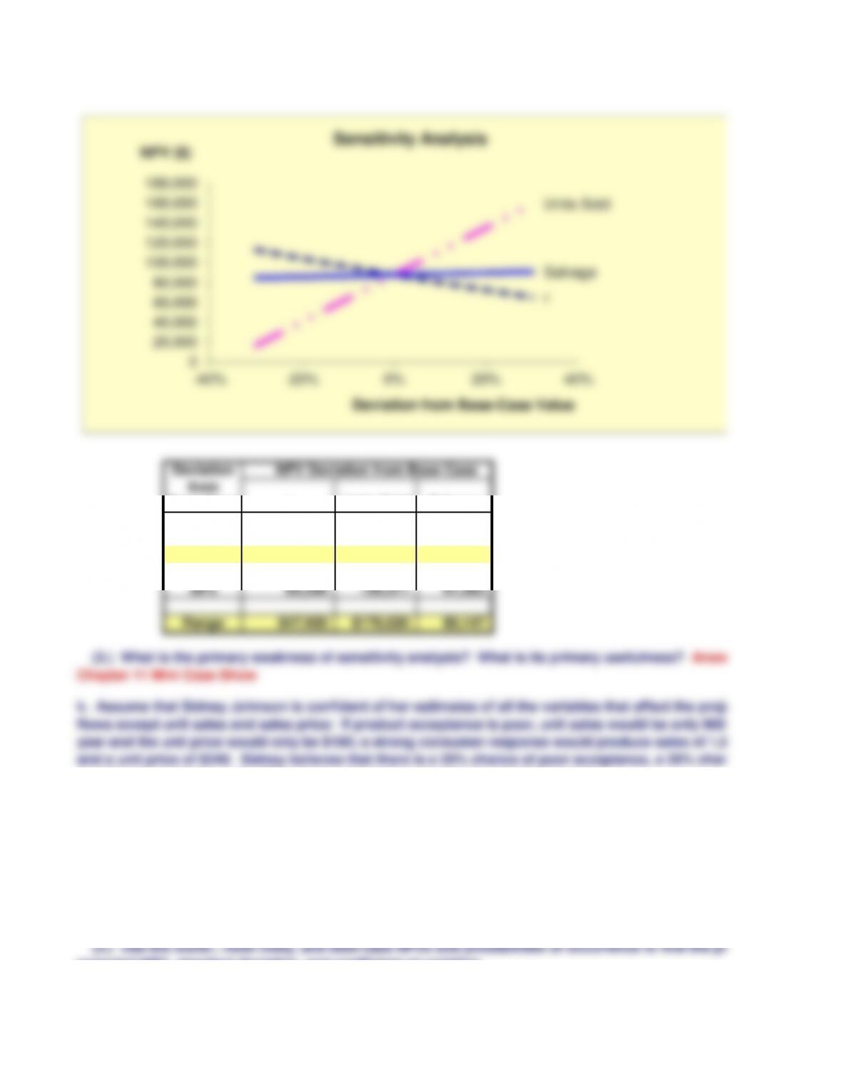
Deviation NPV Deviation from Base Case
from
Base Case r Units Sold Salvage
-30% $113,270 $16,649 $84,936
-15% 100,291 52,329 86,473
0% 88,010 88,010 88,010
15% 76,378 123,690 89,546
30% 65,350 159,371 91,083
Range $47,920 $176,020 $6,147
k. Assume that Sidney Johnson is confident of her estimates of all the variables that affect the project’s cash
flows except unit sales and sales price: If product acceptance is poor, unit sales would be only 900 un
year and the unit price would only be $160; a strong consumer response would produce sales of 1,60
and a unit price of $240. Sidney believes that there is a 25% chance of poor acceptance, a 25% chance of
excellent acceptance, and a 50% chance of average acceptance (the base case).
(1.) What is scenario analysis?
(3.) What is the primary weakness of sensitivity analysis? What is its primary usefulness? Answer
Chapter 11 Mini Case Show
(2.) What is the worst-case NPV? The best-case NPV?
(3.) Use the worst-, most likely, and best-case NPVs and probabilities of occurrence to find the project’s
expected NPV, standard deviation, and coefficient of variation.
Scenario analysis extends risk analysis in two ways: (1) It allows us to change more than one variable a
time, hence to see the combined effects of changes in several variables on NPV, and (2) it allows us to
in the probabilities of changes in the key variables.
r
Units Sold
Salvage
0
20,000
40,000
60,000
80,000
100,000
120,000
140,000
160,000
180,000
-40% -20% 0% 20% 40%
NPV ($)
Deviation from Base-Case Value
Sensitivity Analysis
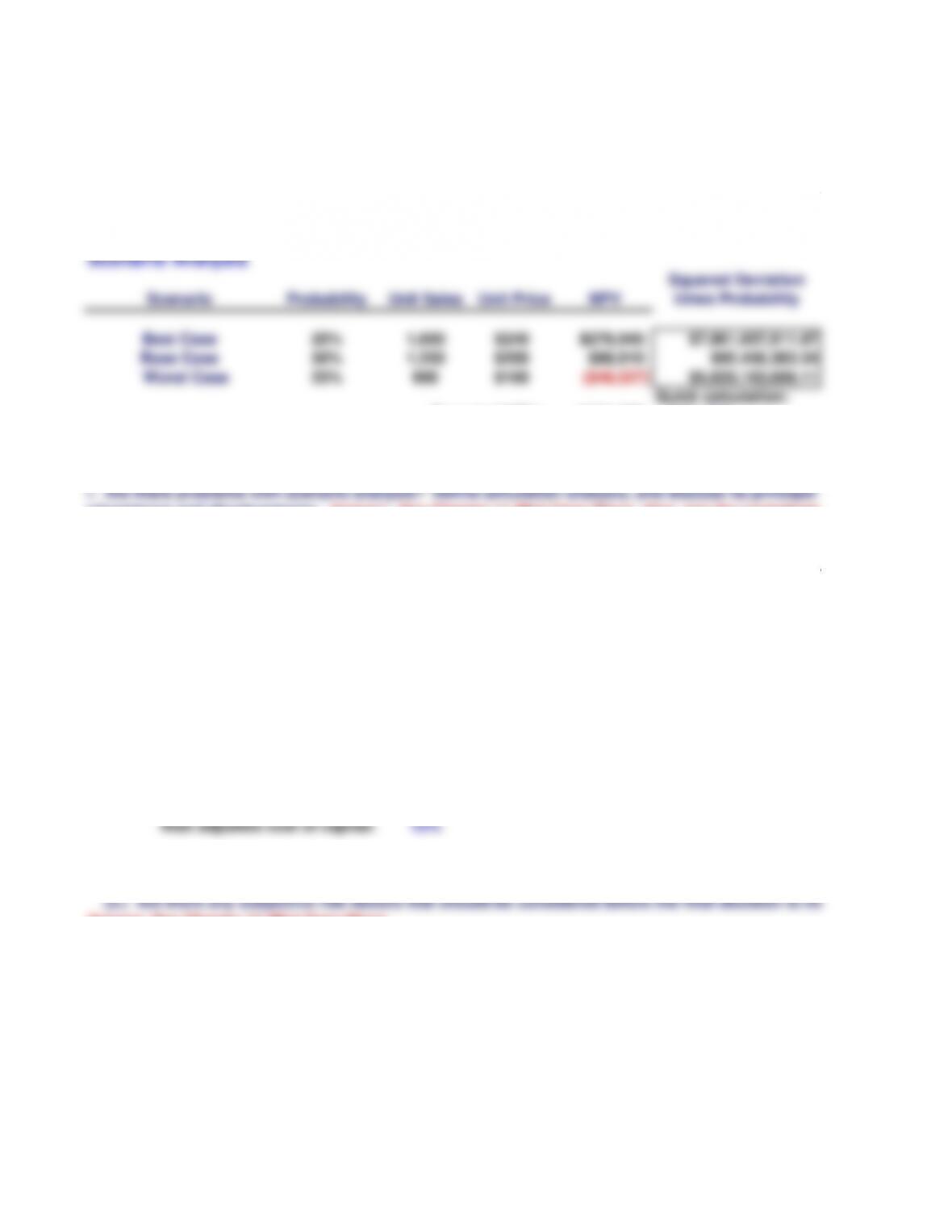
Scenario Analysis
Probability Unit Sales Unit Price NPV
25% 1,600 $240 $278,940
50% 1,250 $200 $88,010
25% 900 $160 ($48,527)
Quick calculation:
Expected NPV = $101,608 $101,608
Standard Deviation = $116,573 $116,573
Coefficient of Variation = Std Dev / Expected NPV = 1.15
$7,861,657,811.87
Squared Deviation
times Probability
$92,456,383.34
$5,635,163,606.11
Best Case
Scenario
Base Case
Worst Case
We could find the NPV by entering the value of unit sales and price for each scenario and then recordin
NPV (this is what we did for the table below). Alternatively, we could use Tools, Scenarios to define t
for each scenario, which we did and show in the Scenario Summary Tab below. In fact, you could ev
Tools, Scenarios, and then click the Summary button on the dialog box, and it will automatically crea
similar to the one below. This is a powerful feature of Excel, and we encourage you to explore it.

10/28/2015
dgeting
ould be set
up in unused space in Shrieves' main plant. The machinery’s invoice price would be approximately $200,000,
install the
ax ruling that
alue of
al cost of
ear. The sales
e new line,
the firm’s net working capital would have to increase by an amount equal to 12% of sales revenues. The firm’s
capital for
a. Define “incremental cash flow.”
uld this be
nswer: See
. Should this
(4.) Finally, assume that the new product line is expected to decrease sales of the firm’s other lines by
er 11 Mini

n net
al
include
Year 4
$89,068
32,782
15,000
$136,850
4
$136,850
102,113
143,984
141,215
$524,162
4
$136,850
$184,772
age project cost of
capital, what are the project’s NPV, IRR, MIRR, PI, payback, and discounted payback? Do these indicators
use the MIRR
NPV
$88,010
$84,936
$86,473
$88,010
$89,546
$91,083
apter 11 Mini
ini Case
e project.
d minus
er: See
h. What does the term ”risk” mean in the context of capital budgeting; to what extent can risk be quantified;
l data or on
he expected
e will actually
orse-than-
an expected,
umed inputs
Excel to
ACC
analys as shown
LVAGE


