Unlock document.
This document is partially blurred.
Unlock all pages and 1 million more documents.
Get Access
g. Now suppose the cost of the project is $75 million and the project cannot be
delayed. But if Tropical Sweets implements the project, then Tropical Sweets
will have a growth option. It will have the opportunity to replicate the original
project at the end of its life. What is the total expected NPV of the two projects if
both are implemented?
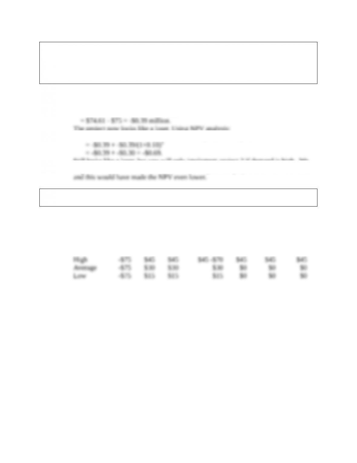
Answer: Suppose the cost of the project is $75 million instead of $70 million, and there is no
option to wait.
NPV = PV of future cash flows - cost
The project now looks like a loser. Using NPV analysis:
NPV = NPV Of Original Project + NPV Of Replication Project
Still looks like a loser, but you will only implement project 2 if demand is high. We
might have chosen to discount the cost of the replication project at the risk-free rate,
h. Tropical Sweets will replicate the original project only if demand is high. Using
decision tree analysis, estimate the value of the project with the growth option.
Answer: The future cash flows of the optimal decisions are shown below. The cash flow in
year 3 for the high demand scenario is the cash flow from the original project and the
cost of the replication project.
0 1 2 3 4 5 6
Mini Case: 26 - 1
© 2017 Cengage Learning. All Rights Reserved. May not be scanned, copied or duplicated, or posted to a publicly accessible
website, in whole or in part.
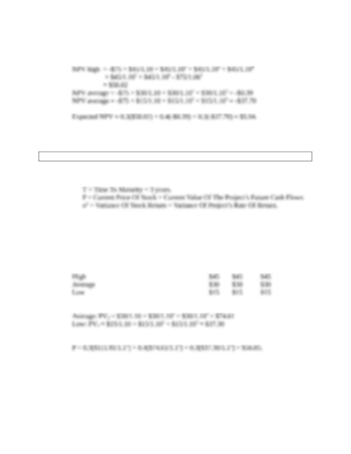
To find the NPV, we discount the risky cash flows at the 10 percent cost of capital,
and the non-risky cost to replicate (i.e., the $75 million) at the risk-free rate.
Thus, the option to replicate adds enough value that the project now has a positive
NPV.
i. Use a financial option model to estimate the value of the growth option.
Answer: X = Strike Price = Cost Of Implement Project = $75 million.
RRF = Risk-Free Rate = 6%.
We explain how to calculate P and σ2 below.
Step 1: Find the value of all cash flows beyond the exercise date discounted back to
the exercise date. Here is the time line. The exercise date is year 1, so we discount
all future cash flows back to year 3.
012345 6
High: PV3 = $45/1.10 + $45/1.102 + $45/1.103 = $111.91
The current expected present value, P, is:
Mini Case: 26 - 2
© 2017 Cengage Learning. All Rights Reserved. May not be scanned, copied or duplicated, or posted to a publicly accessible
website, in whole or in part.
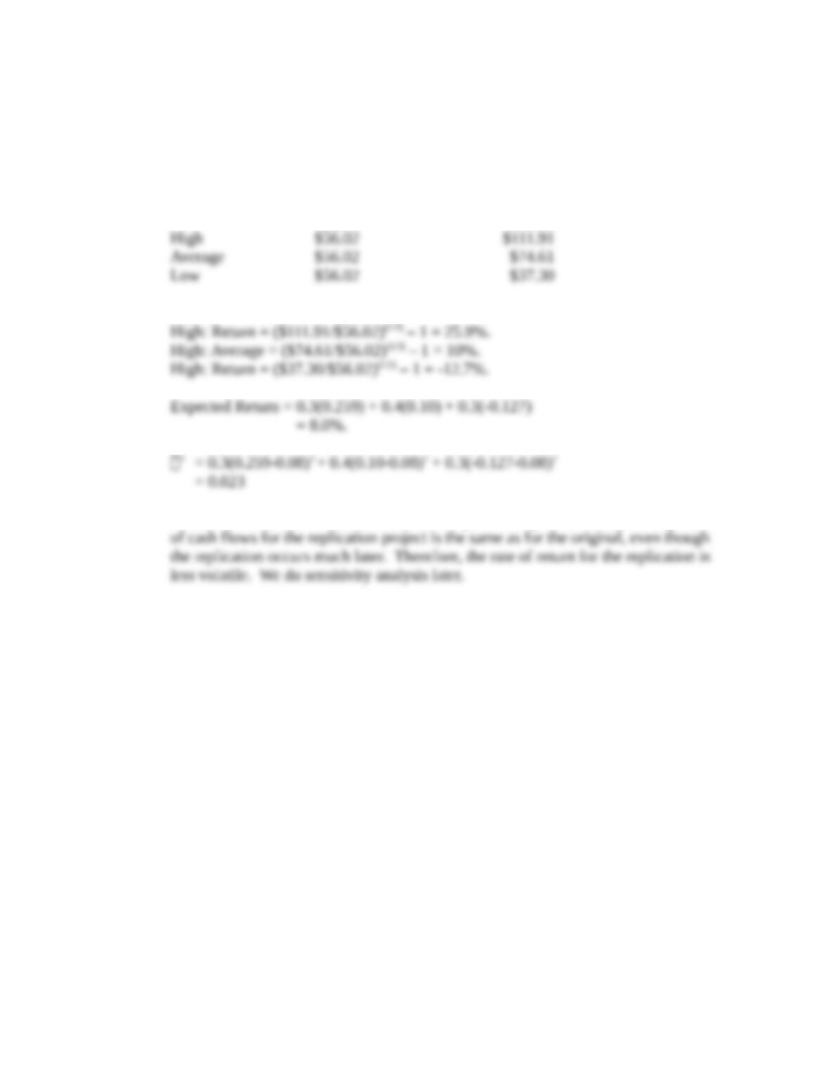
Direct approach for estimating σ2:
From our previous analysis, we know the current value of the project and the value
for each scenario at the time the option expires (year 3). Here is the time line:
Current Value Value At Expiration
Year 0 Year 3
The annual rate of return is:
This is lower than the variance found for the previous option because the dispersion
Mini Case: 26 - 3
© 2017 Cengage Learning. All Rights Reserved. May not be scanned, copied or duplicated, or posted to a publicly accessible
website, in whole or in part.
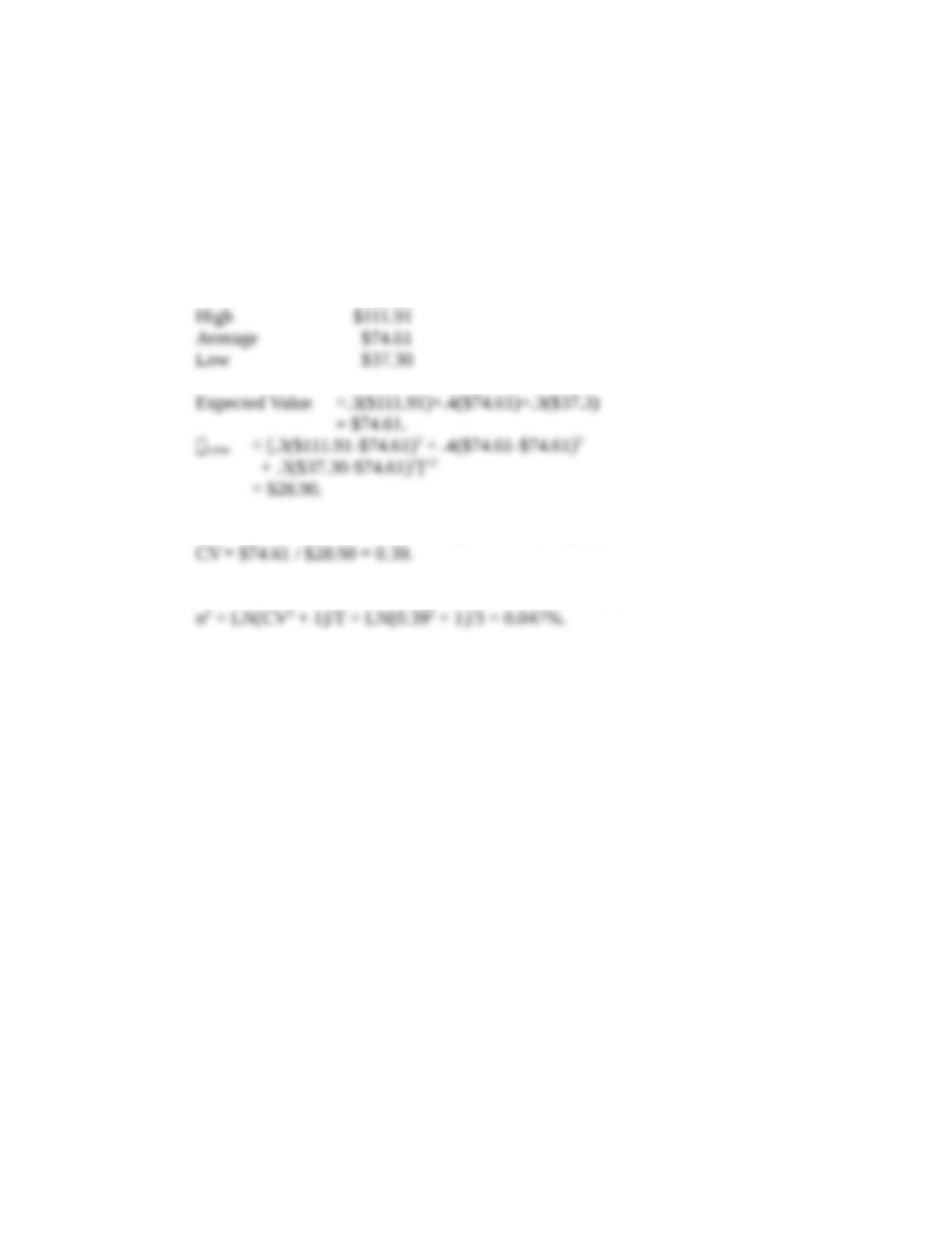
The indirect approach:
First, find the coefficient of variation for the value of the project at the time the option
expires (year 3).
We previously calculated the value of the project at the time the option expires, and
we can use this to calculate the expected value and the standard deviation.
Value At Expiration
Year 3
Coefficient of Variation = CV = Expected Value / value
To find the variance of the project’s rate or return, we use the formula below:
Mini Case: 26 - 4
© 2017 Cengage Learning. All Rights Reserved. May not be scanned, copied or duplicated, or posted to a publicly accessible
website, in whole or in part.
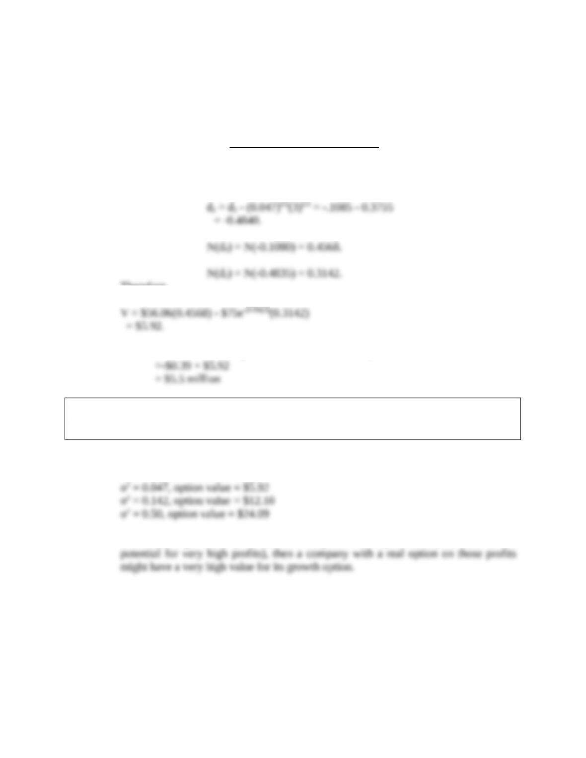
Now, we proceed to use the OPM:
V = $56.06[N(d1)] - $75e-(0.06)(3)[N(d2)].
d1 =
5.0
)3(
5.0
)047.0(
)3)](0.047/206.0[()$56.06/$75ln(
= -0.1085.
d2 = d1 - (0.047)0.5(3)0.5 = -.1085 - 0.3755
= -0.4840.
N(d1) = N(-0.1080) = 0.4568.
N(d2) = N(-0.4835) = 0.3142.
Therefore,
Total Value = NPV Of Project 1 + Value Of Growth Option
j. What happens to the value of the growth option if the variance of the project’s
return is 0.142? What if it is 0.50? How might this explain the high valuations
of many dot.com companies?
Answer: If risk, defined by σ2, goes up, then value of growth option goes up (see the file Ch26
mini case.xls for calculations):
If the future profitability of dot.com companies is very volatile (i.e., there is the
Mini Case: 26 - 5
© 2017 Cengage Learning. All Rights Reserved. May not be scanned, copied or duplicated, or posted to a publicly accessible
website, in whole or in part.


