Chapter 26
Real Options
ANSWERS TO END-OF-CHAPTER QUESTIONS
26-1 a. Real options occur when managers can influence the size and risk of a project’s cash
flows by taking different actions during the project’s life. They are referred to as real
b. Investment timing options give companies the option to delay a project rather than
implement it immediately. This option to wait allows a company to reduce the
uncertainty of market conditions before it decides to implement the project. Capacity
26-2 Postponing the project means that cash flows come later rather than sooner; however,
SOLUTIONS TO END-OF-CHAPTER PROBLEMS
26-1 a. 0 1 2 20
├─────┼─────┼────── ────┤
-20 3 3 3
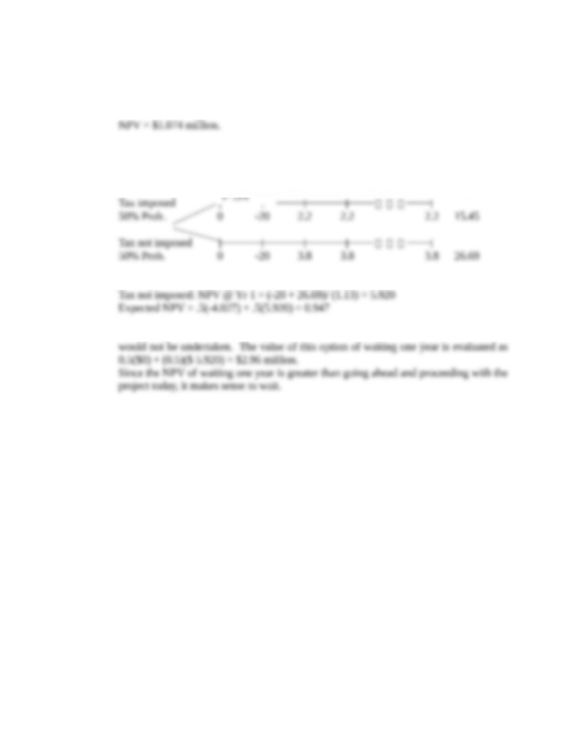
b. Wait 1 year:
PV @
0 1 2 3 21 Yr. 1
Tax imposed: NPV @ Yr. 1 = (-20 + 15.45)/(1.13) = -4.027
Note though, that if the tax is imposed, the NPV of the project is negative and therefore
r= 13%
26-2 a. 0 1 2 3 4
├─────┼─────┼─────┼─────┤
-8 4 4 4 4
NPV = $4.6795 million.
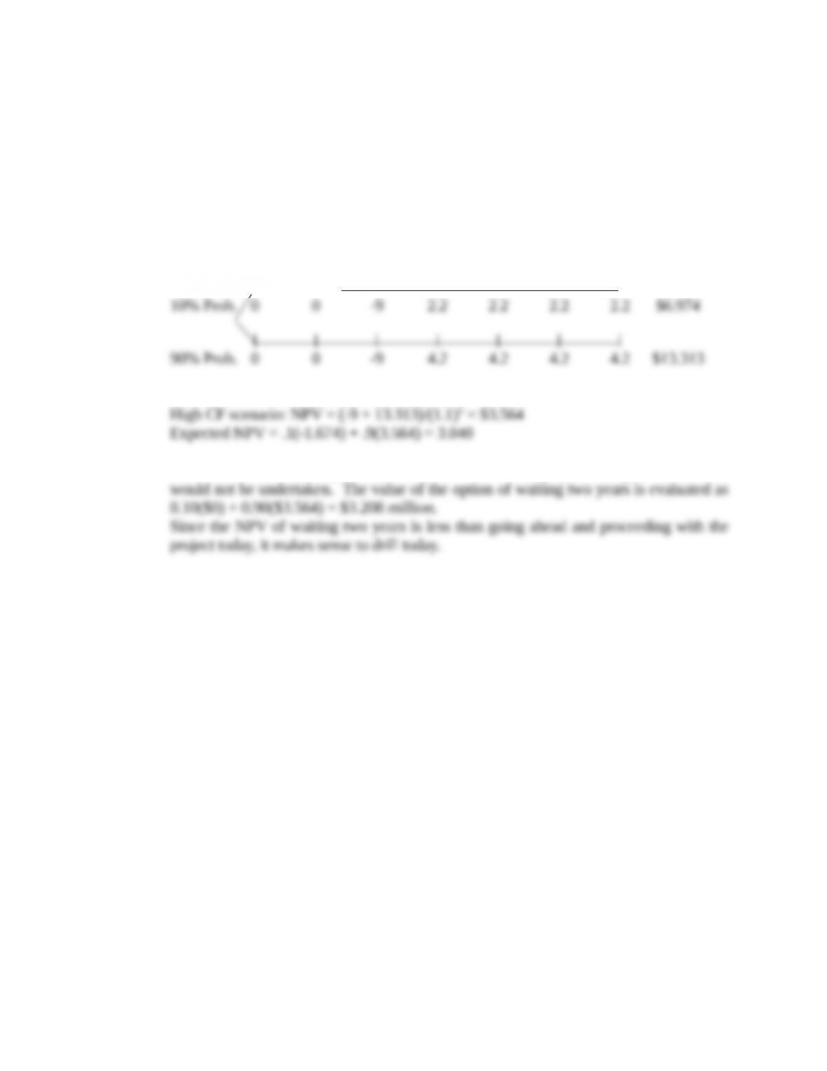
b. Wait 2 years:
PV @
0 1 2 3 4 5 6 Yr. 2
|||||||
Low CF scenario: NPV = (-9 + 6.974)/(1.1)2 = -$1.674
If the cash flows are only $2.2 million, the NPV of the project is negative and, thus,
10%
r = 10%
b. Wait 1 year:
NPV @
If the cash flows are only $30 million per year, the NPV of the project is negative.
However, we’ve not considered the fact that the company could then be sold for $280
million. The decision tree would then look like this:
NPV @
million.
Given the option to sell, it makes sense to wait 1 year before deciding whether to
make the acquisition.
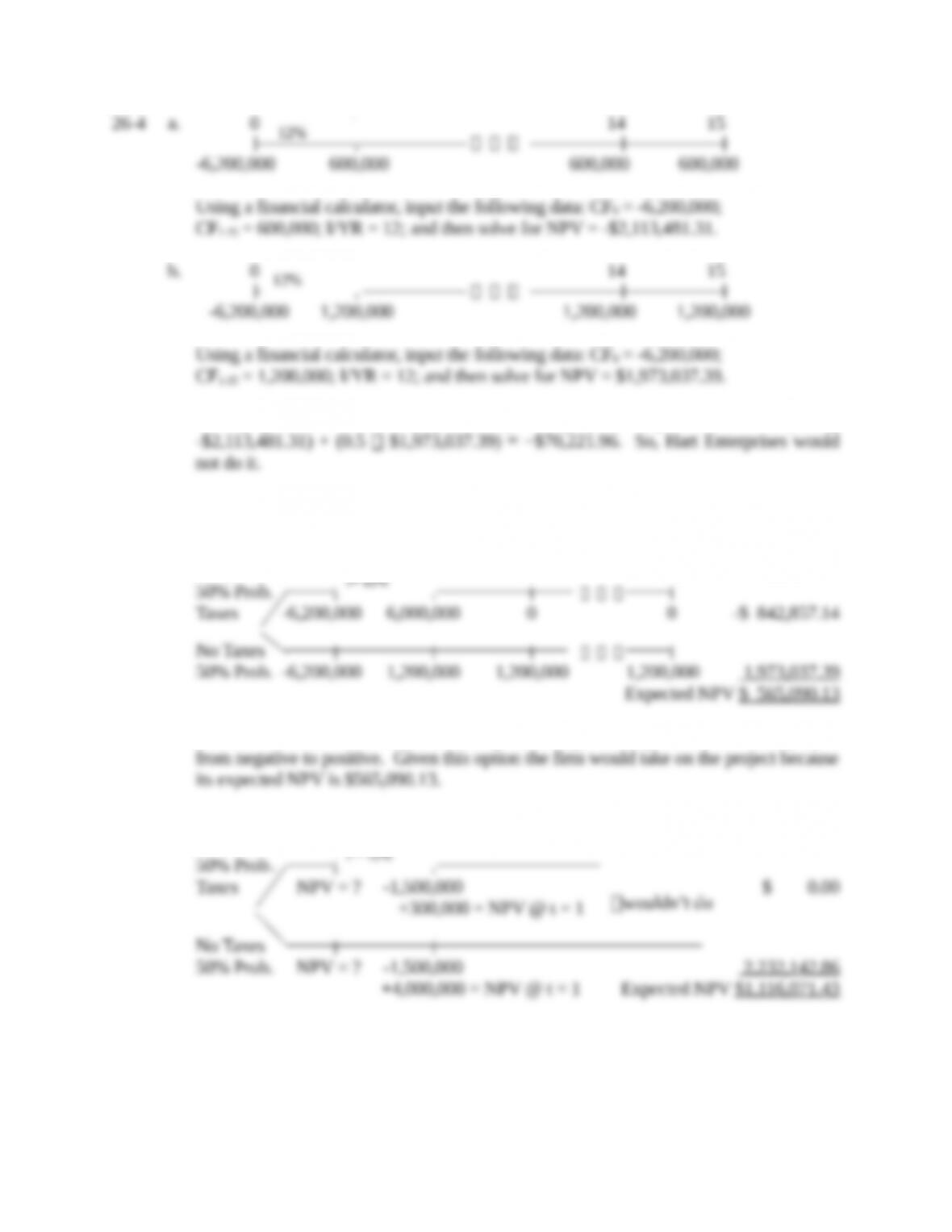
c. If they proceed with the project today, the project’s expected NPV = (0.5
d. Since the project’s NPV with the tax is negative, if the tax were imposed the firm
would abandon the project. Thus, the decision tree looks like this:
NPV @
0 1 2 15 Yr. 0
Yes, the existence of the abandonment option changes the expected NPV of the project
e. NPV @
0 1 Yr. 0
If the firm pays $1,116,071.43 for the option to purchase the land, then the NPV of the
project is exactly equal to zero. So the firm would not pay any more than this for the
option.
r= 12%
r = 12%
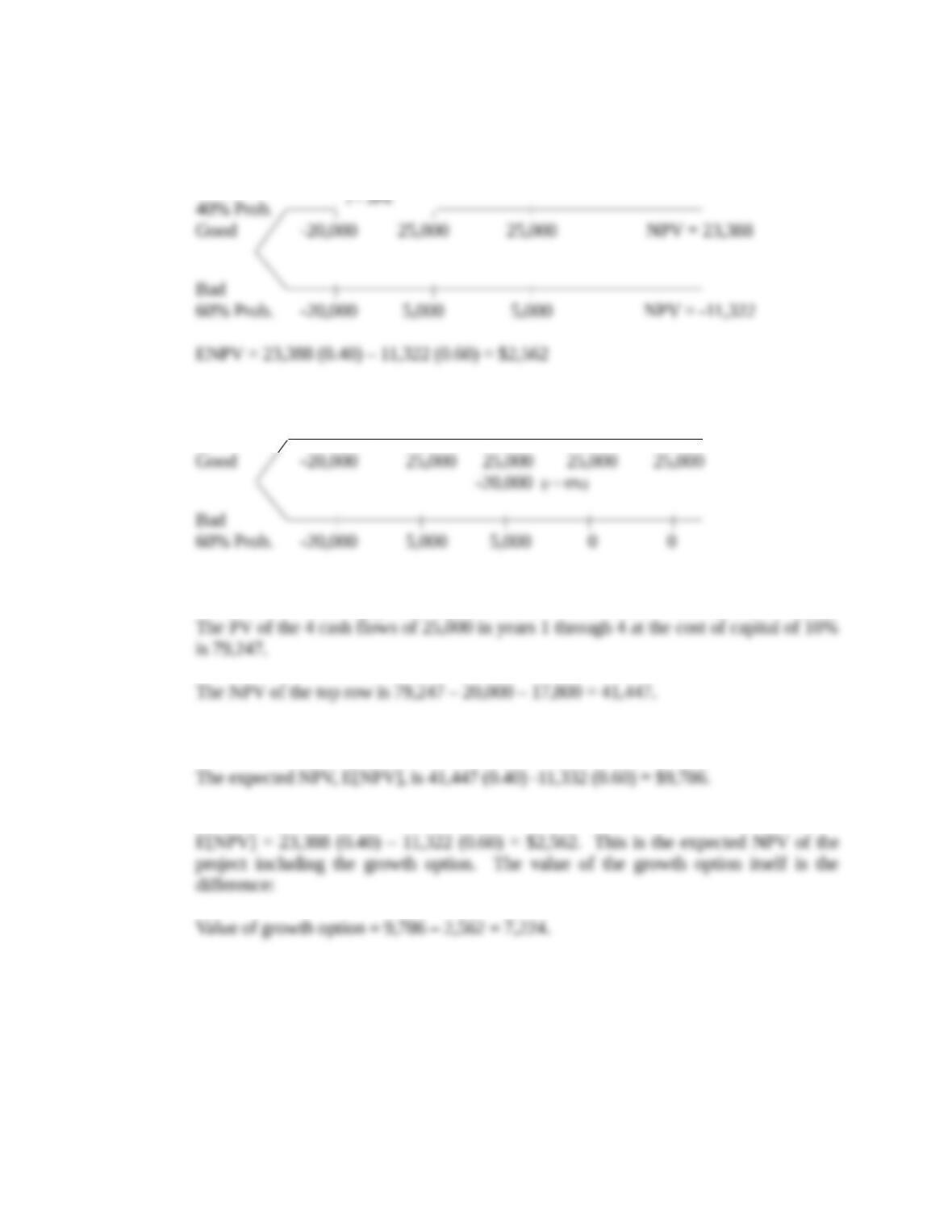
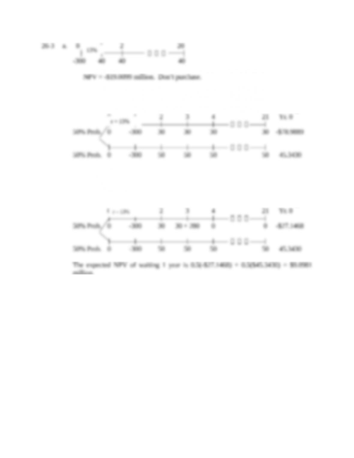
26-5
a.
012
b.
01234
40% Prob.|||||
The PV of the 20,000 payment in year 2 at the risk free rate is 20,000/(1.06)2 = 17,800.
The NPV of the bottom row is still -11,332, as it was in part a.
r = 10%
r = 10%
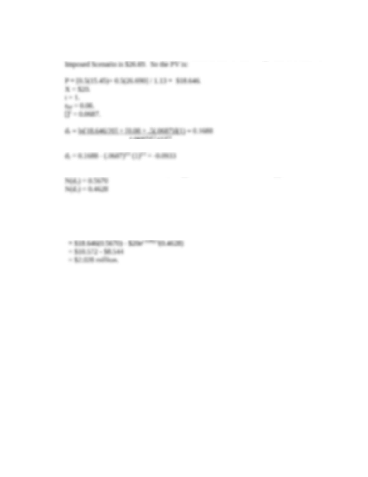
26-6 P = PV of all expected future cash flows if project is delayed. From Problem 14-1 we
know that PV @ Year 1 of Tax Imposed scenario is $15.45 and PV @ Year 1 of Tax Not
(.0687)0.5 (1)0.5
From Excel function NORMSDIST, or approximated from the table in Appendix A:
Using the Black-Scholes Option Pricing Model, you calculate the option’s value as:
V = P[N(d1)] –
tr
RF
Xe
[N(d2)]
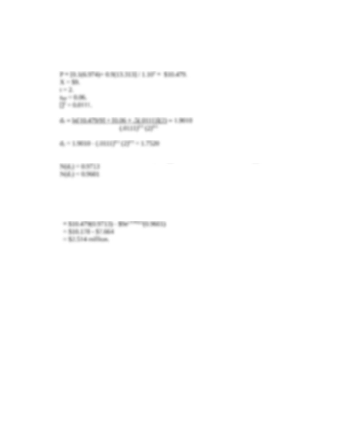
26-7 P = PV of all expected future cash flows if project is delayed. From Problem 26-1 we
know that PV @ Year 2 of Low CF Scenario is $6.974 and PV @ Year 2 of High CF
Scenario is $13.313. So the PV is:
From Excel function NORMSDIST, or approximated from the table in Appendix A:
Using the Black-Scholes Option Pricing Model, you calculate the option’s value as:
V = P[N(d1)] –
tr
RF
Xe
[N(d2)]