
Chapter 7
Sampling and Sampling Distributions
Learning Objectives
1. Understand the importance of sampling and how results from samples can be used to provide
estimates of population characteristics such as the population mean, the population standard
deviation and / or the population proportion.
2. Know what simple random sampling from a finite population is and how simple random samples are
selected.
3. Understand how to select a random sample from an infinite population.
4. Understand the concept of a sampling distribution.
5. Understand the central limit theorem and the important role it plays in sampling.
6. Specifically know the characteristics of the sampling distribution of the sample mean (
x
) and the
sampling distribution of the sample proportion (
p
).
7. Learn about a variety of sampling methods including stratified random sampling, cluster sampling,
systematic sampling, convenience sampling and judgment sampling.
8. Know the definition of the following terms:
parameter target population
sampled population sampling distribution
sample statistic finite population correction factor
simple random sampling standard error
point estimator central limit theorem
point estimate unbiased
Solutions:
1. a. AB, AC, AD, AE, BC, BD, BE, CD, CE, DE
b. With 10 samples, each has a 1/10 probability.
c. B and D because the two smallest random numbers are .0476 and .0957.
6. a. Finite population. A frame could be constructed obtaining a list of licensed drivers from the New
York state driver’s license bureau.
b. Sampling from an infinite population. The sample is taken from the production line producing boxes
of cereal.
7. a.
x x n
i
= = = /54
69
b.
sx x
n
i
=−
−
( )2
1
( )x x
i−2
= (–4)2 + (-1)2 + 12 (-2)2 + 12 + 52 = 48
48
9. a.
x x n
i
= = = /465
593
b.
xi
( )x x
i−
( )x x
i−2
94
+1
1
100
+7
49
85
-8
64
94
+1
1
92
-1
1
Totals
465
0
116
sx x
n
i
=−
−= =
( ) .
2
1
116
4539
10. a. Two of the 40 stocks in the sample received a 5 Star rating.
2.05
40
p==
b. Seventeen of the 40 stocks in the sample are rated Above Average with respect to risk.
17 .425
40
c. There are eight stocks in the sample that are rated 1 Star or 2 Star.
p==
8.20
40
11. a.
816 68
12
i
x
xn
= = =
b.
2
() 3522 17.8936
1 12 1
i
xx
sn
−
= = =
−−
12. a. The sampled population is U. S. adults that are 50 years of age or older.
b. We would use the sample proportion for the estimate of the population proportion.
350 .8216
426
p==
c. The sample proportion for this issue is .74 and the sample size is 426.
354 .8310
426
p==
e. The inferences in parts (b) and (d) are being made about the population of U.S. adults who are age
50 or older. So, the population of U.S. adults who are age 50 or older is the target population. The
target population is the same as the sampled population. If the sampled population was restricted to
members of AARP who were 50 years of age or older, the sampled population would not be the
13. a.
p
= 454/478 = .9498
b.
p
= 741/833 = .8896
p
e.
p
=(454 + 741 + 1058)/(478 + 833 + 1644) = .7624
manager and select managers associated with the 50 smallest random numbers as the sample.
b. Use Excel’s AVERAGE function to compute the mean for the sample.
c. Use Excel’s STDEV.S function to compute the sample standard deviation.
E
()x
=
= 200
/ 50 / 100 5
xn
= = =
For 5,
195 205x
Using Standard Normal Probability Table:
x
51
x
x
−
Using Standard Normal Probability Table:
At
x
= 210,
zx
x
=−= =
10
52
( 2)Pz
= .9772
At
x
= 190,
10 2
5
x
x
z
−−
= = = −
( 2)Pz−
= .0228
25/ 50 3.54
x
==
25/ 100 2.50
x
==
25/ 150 2.04
x
==
x
At
x
= 52,300,
52,300 51,800 .97
516.40
z−
==
P(
x
≤ 52,300) = P(z ≤ .97) = .8340
At
x
= 51,300,
51,300 51,800 .97
516.40
z−
= = −
P(
x
< 51,300) = P(z < -.97) = .1660
x
x
x
x
x
x
18.0 17.5 .88
P(17.0 ≤
x
≤ 18.0) = .8106 – .1894 = .6212
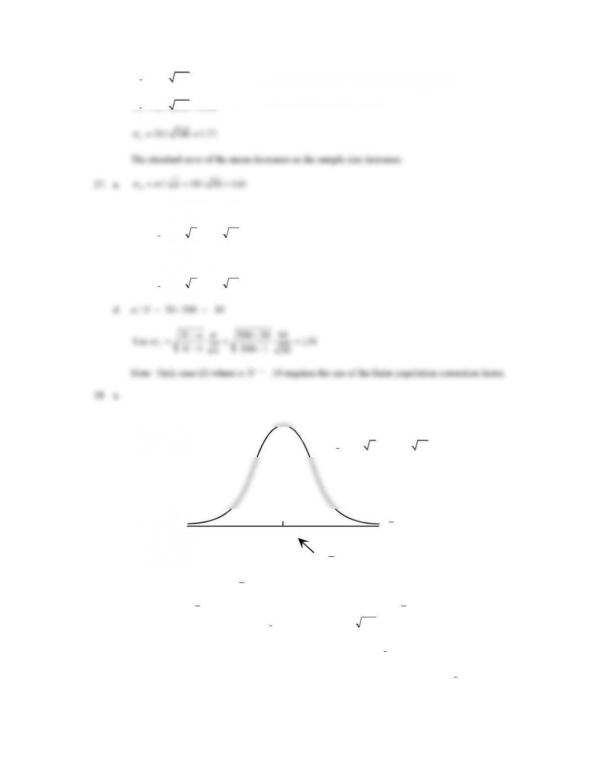
21.
/ 100/ 90 10.54
xn
= = =
This value for the standard error can be used for parts (a) and (b)
below.
492 502 .95
10.54
z−
= = −
P(z < -.95) = .1711
probability = .8289 – .1711 = .6578
Using Excel: NORM.DIST(512,502,10.54,TRUE)-NORM.DIST(492,502,10.54,TRUE) = .6573
525 515 .95
10.54
505 515 .95
10.54
z−
= = −
P(z < -.95) = .1711
probability = .8289 – .1711 = .6578
Using Excel: NORM.DIST(525,515,10.94,TRUE)-NORM.DIST(505,515,10.54,TRUE) = .6573
The probability of being within 10 of the mean on the Mathematics portion of the test is exactly the
Within
200 means
x
– 16,642 must be between -200 and +200.
The z value for
x
– 16,642 = -200 is the negative of the z value for
x
– 16,642 = 200. So we just
show the computation of z for
x
– 16,642 = 200.
n = 30
200 .46
2400 / 30
z==
P(-.46 ≤ z ≤ .46) = .6772 – .3228 = .3544
Using Excel: NORM.DIST(16842,16642,2400/SQRT(30),TRUE)-
NORM.DIST(-16442,16642,2400/SQRT(30),TRUE) = .3519
200 .59
2400 / 50
Using Excel: NORM.DIST(16842,16642,2400/SQRT(50),TRUE)-
NORM.DIST(16442,16642,2400/SQRT(50),TRUE) = .4443
n = 100
200 .83
2400 / 100
z==
P(-.83 ≤ z ≤ .83) = .7967 – .2033 = .5934