50. N = 60 n = 10
a. r = 20 x = 0
( )
20 40 40!
1
0 10 10!30!
10
c. 1 – f (0) – f (1) = 1 – .0112 – .0725 = .9163 ≈ .92
d. Same as the probability one will be from Hawaii. In part b that was found to equal approximately
.07.
5 10
03 (1)(120)
37 3! 7!
03 0!3! 3!4!
10
3!7!
3
This is the probability there will be no banks with increased lending in the study.
b. n = 3, x = 3
37 3! 7!
30 3!0! 0!7!
10
3!7!
3
This is the probability there all three banks with increased lending will be in the study. This has a
very low probability of happening.
c. n = 3, x = 1
37 3! 7!
12 1!2! 2!5!
(1) 10!
10
3!7!
3
f
= = =
HYPGEOM.DIST(1,3,3,10,FALSE) = .5250
n = 3, x = 2
37 3! 7!
21 2!1! 1!6!
x
f(x)
0
0.2917
1
0.5250
2
0.1750
3
0.0083
Total
1.0000
f(1) = .5250 has the highest probability showing that there is over a .50 chance that there will be
exactly one bank that had increased lending in the study.
d. P(x > 1) =
1 (0) 1 .2917 .7083f− = − =
There is a reasonably high probability of .7083 that there will be at least one bank that had increased
10

2
2
3 3 10 3
1 3 1 .49
1 10 10 10 1
.49 .70
r r N n
nN N N
−−
= − = − =
−−
= = =
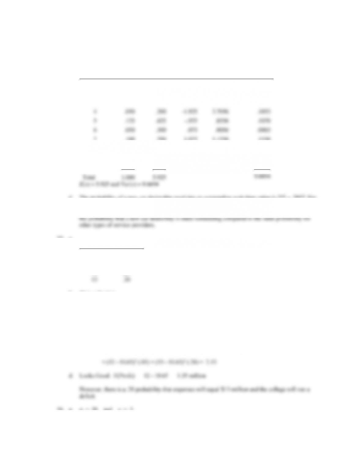
53. a. The probability distribution for x follows.
x
f (x)
0
.0960
1
.5700
2
.2380
3
.0770
4
.0190
Total
1.0000
b. and c follow.
x
f (x)
xf (x)
x –
(x –
)2
(x –
)2 f (x)
0
.0960
.0000
-1.3530
1.8306
.1757
1
.5700
.5700
-.3530
.1246
.0710
2
.2380
.4760
.6470
.4186
.0996
3
.0770
.2310
1.6470
2.7126
.2089
4
.0190
.0760
2.6470
7.0066
.1331
Total
1.0000
1.3530
0.6884
E(x) = 1.353, Var(x) = .6884,
.6884 .8297==
d. The expected value of 1.353 indicates that the mean wind condition when an accident occurred is
slightly greater than light wind conditions.
54. a.
x
f (x)
1
.150
2
.050
3
.075
4
.050
5
.125
6
.050
7
.100
8
.125
9
.125
10
.150
Total
1.000
b. Probability of outstanding service is .125 + .150 = .275
c.
x
f (x)
xf (x)
x –
(x –
)2
(x –
)2 f (x)
1
.150
.150
-4.925
24.2556
3.6383
2
.050
.100
-3.925
15.4056
.7703
3
.075
.225
-2.925
8.5556
.6417
4
.050
.200
-1.925
3.7056
.1853
5
.125
.625
-.925
.8556
.1070
6
.050
.300
.075
.0056
.0003
7
.100
.700
1.075
1.1556
.1156
8
.125
1.000
2.075
4.3056
.5382
9
.125
1.125
3.075
9.4556
1.1820
10
.150
1.500
4.075
16.6056
2.4908
Total
1.000
5.925
9.6694
d. The probability of a new car dealership receiving an outstanding wait-time rating is 2/7 = .2857. For
the remaining 40 – 7 = 33 service providers, 9 received and outstanding rating; this corresponds to a
probability of 9/33 = .2727. For these results, there does not appear to be much difference between
55. a.
x
f (x)
9
.30
10
.20
11
.25
12
.05
13
.20
b. E(x) = x f (x)
= 9(.30) + 10(.20) + 11(.25) + 12(.05) + 13(.20) = 10.65
Expected value of expenses: $10.65 million
c. Var(x) = (x –
)2 f (x)
= (9 – 10.65)2 (.30) + (10 – 10.65)2 (.20) + (11 – 10.65)2 (.25)
56. a. n = 20 and x = 3
3 17
20
b. n = 20 and x = 0
(x 5) (0) (1) (2) (3) (4) (5)P f f f f f f = + + + + +
= BINOM.DIST(5,20,.28,TRUE) = .4952
c. E(x) = n p = 2000(.49) = 980
57. a. We must have E(x) = np 25
For the 18-34 age group, p = .16.
n(.16) 25
n 156.25
For the 18-34 age group you need to sample at least 157 people to have an expected number of at
c. For the 65 and over age group, p = .02.
n(.02) 25
n 1250
For the 65 and over age group you need to sample at least 1250 people to have an expected number
use the binomial probability distribution.
a. n = 5
05
5
(0) (0.01) (0.99)
0
f
=
= BINOM.DIST(0,5,.01,FALSE) = .9510
59. a. E(x) = np = 100(.041) = 4.1
60. a. E(x) = 200(.235) = 47
b.
(1 ) 200(.235)(.765) 5.9962np p= − = =
c. For this situation p = .765 and (1-p) = .235; but the answer is the same as in part (b). For a binomial
61.
= 15
Probability of 20 or more arrivals = f (20) + f (21) + · · ·
62.
= 1.5
Probability of 3 or more breakdowns is 1 – [ f (0) + f (1) + f (2) ].
63.
= 10 f (4) = POISSON.DIST(4,10,FALSE) = .0189
64. a.
33
3
(3) 3!
e
f−
=
= POISSON.DIST(3,3,FALSE) = .2240
14
5
b. f (3) + f (4) + · · · = 1 – [ f (0) + f (1) + f (2) ]
65. Hypergeometric N = 52, n = 5 and r = 4.
a.
4 48
23 6(17296)
52 2,598,960
5
=
= HYPGEOM.DIST(2,5,4,52,FALSE) = .0399
4 48
14 4(194580)
52 2,598,960
5
=
c.
4 48
05 1,712,304
52 2,598,960
5
=
= HYPGEOM.DIST(0,5,4,52,FALSE) = .6588
d. 1 – f (0) = 1 – .6588 = .3412
66. a. Hypergeometric distribution with N = 10, n =2, and r = 7.
7 10 7
1 2 1
(1) 10
2
r N r
x n x
fN
n
−−
−−
= = =
HYPGEOM.DIST(1,2,7,10,FALSE) = .4667
73
20
2
f (0) = 30 e-3
0! = e-3 = .0498

73
02