Chapter 5
Discrete Probability Distributions
Learning Objectives
1. Understand the concepts of a random variable and a probability distribution.
2. Be able to distinguish between discrete and continuous random variables.
3. Be able to compute and interpret the expected value, variance, and standard deviation for a discrete
random variable.
4. Be able to compute and work with probabilities involving a binomial probability distribution.
5. Be able to compute and work with probabilities involving a Poisson probability distribution.
6. Know when and how to use the hypergeometric probability distribution.
Solutions:
1. a. Head, Head (H,H)
Head, Tail (H,T)
b. x = number of heads on two coin tosses
c.
Outcome
Values of x
(H,H)
2
(H,T)
1
(T,H)
1
(T,T)
0
d. Discrete. It may assume 3 values: 0, 1, and 2.
2. a. Let x = time (in minutes) to assemble the product.
3. Let Y = position is offered
N = position is not offered
c.
Experimental Outcome
(Y,Y,Y)
(Y,Y,N)
(Y,N,Y)
(N,Y,Y)
(Y,N,N)
(N,Y,N)
(N,N,Y)
(N,N,N)
Value of N
3
2
2
2
1
1
1
0
5. a. S = {(1,1), (1,2), (1,3), (2,1), (2,2), (2,3)}
b.
Experimental Outcome
(1,1)
(1,2)
(1,3)
(2,1)
(2,2)
(2,3)
Number of Steps Required
2
3
4
3
4
5
6. a. values: 0,1,2,…,20
discrete
b. values: 0,1,2,…
discrete
7. a. f (x) 0 for all values of x.
f (x) = 1 Therefore, it is a proper probability distribution.
8. a.
x
f (x)
1
3/20 = .15
2
5/20 = .25
3
8/20 = .40
4
4/20 = .20
Total 1.00
b.
c. f (x) 0 for x = 1,2,3,4.
9. a. There are a total of 26,975 unemployed persons in the data set. Each probability f(x) is computed by
dividing the number of months of unemployment by 26,975. For example, f (1) = 1029/26,975 =
.0381. The complete probability distribution is as follows.
x
f (x)
1
.0381
2
.0625
3
.0841
4
.0992
5
.1293
6
.1725
7
.1537
8
.1330
9
.0862
10
.0415
b.
( ) 0 and ( ) 1f x f x=
c. Probability 2 months or less = f (1) + f (2) = .0381 + .0625 = .1006
10. a.
x
f (x)
1
0.05
2
0.09
3
0.03
4
0.42
5
0.41
1.00
b.
x
f (x)
1
0.04
2
0.10
3
0.12
4
0.46
5
0.28
1.00
c. P(4 or 5) = f (4) + f (5) = 0.42 + 0.41 = 0.83
11. a.
Duration of Call
x
f (x)
1
0.25
2
0.25
3
0.25
4
0.25
1.00
b.
c. f (x) 0 and f (1) + f (2) + f (3) + f (4) = 0.25 + 0.25 + 0.25 + 0.25 = 1.00
12. a. Yes; f (x) 0. f (x) = 1
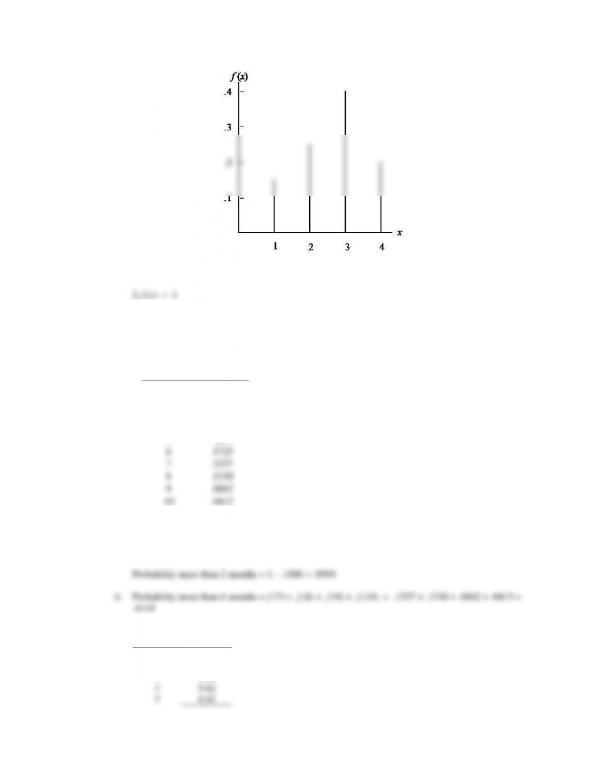
13. a. Yes, since f (x) 0 for x = 1,2,3 and f (x) = f (1) + f (2) + f (3) = 1/6 + 2/6 + 3/6 = 1
0.10
0.20
0.30
f (x)
x
12 3 4
0
14. a. f (200) = 1 – f (-100) – f (0) – f (50) – f (100) – f (150)
= 1 – .95 = .05
This is the probability MRA will have a $200,000 profit.
= .25 + .10 +.05 = .40
15. a.
x
f (x)
x f (x)
3
.25
.75
6
.50
3.00
9
.25
2.25
1.00
6.00
E(x) =
= 6
b.
x
x –
(x –
)2
f (x)
(x –
)2 f (x)
3
-3
9
.25
2.25
6
0
0
.50
0.00
9
3
9
.25
2.25
4.50
Var(x) =
2 = 4.5
c.
=
4.50
= 2.12
16. a.
y
f (y)
y f (y)
2
.2
.4
4
.3
1.2
7
.4
2.8
8
.1
.8
1.0
5.2
E(y) =
= 5.2
b.
y
y –
(y –
)2
f (y)
(y –
)2 f (y)
2
-3.20
10.24
.20
2.048
4
-1.20
1.44
.30
.432
7
1.80
3.24
.40
1.296
8
2.80
7.84
.10
.784
4.560
( ) 4.56
4.56 2.14
Var y
=
==
17. a. Total Student = 1,518,859
x = 1 f(1) = 721,769/1,518,859 = .4752
x = 2 f(2) = 601,325/1,518,859 = .3959
b. P(x > 1) = 1 – f(1) = 1 – .4752 = .5248
c. P(x > 3) = f(3) + f(4) + f(5) = .1098 + .0147 + .0044 = .1289
d./e.
x
f (x)
x f (x)
x –
(x –
)2
(x –
)2 f (x)
1
.4752
.4752
-.6772
.4586
.2179
2
.3959
.7918
.3228
.1042
.0412
3
.1098
.3293
1.3228
1.7497
.1921
4
.0147
.0587
2.3228
5.3953
.0792
5
.0044
.0222
3.3228
11.0408
.0489
1.6772
.5794
E(x) = Σ x f(x) = 1.6772
The mean number of times a student takes the SAT is 1.6772, or approximately
1.7 times.
22
( ) ( ) .5794x f x
= − =
2.5794 .7612
= = =
18. a/b/
x
f (x)
xf (x)
x –
(x –
)2
(x –
)2 f (x)
0
.2188
.0000
-1.1825
1.3982
.3060
1
.5484
.5484
-.1825
.0333
.0183
2
.1241
.2483
.8175
.6684
.0830
3
.0489
.1466
1.8175
3.3035
.1614
4
.0598
.2393
2.8175
7.9386
.4749
Total
1.0000
1.1825
1.0435
E(x)
Var(x)
c/d.
y
f (y)
yf (y)
y –
(y –
)2
(y –
)2 f (y)
0
.2497
.0000
-1.2180
1.4835
.3704
1
.4816
.4816
-.2180
.0475
.0229
2
.1401
.2801
.7820
.6115
.0856
3
.0583
.1749
1.7820
3.1755
.1851
4
.0703
.2814
2.7820
7.7395
.5444
Total
1.0000
1.2180
1.2085
E(y)
Var(y)
e. The expected number of times that owner-occupied units have a water supply stoppage lasting 6 or
more hours in the past 3 months is 1.1825, slightly less than the expected value of 1.2180 for renter–
occupied units. And, the variability is somewhat less for owner-occupied units (1.0435) as compared
19. a. f (x) 0 for all values of x.
f (x) = 1 Therefore, it is a valid probability distribution.
d. Expected value and variance computations follow.
x
f (x)
xf (x)
x –
(x –
)2
(x –
)2 f (x)
10
.05
.5
-33.0
1089.0
54.45
20
.10
2.0
-23.0
529.0
52.90
30
.10
3.0
-13.0
169.0
16.90
40
.20
8.0
-3.0
9.0
1.80
50
.35
17.5
7.0
49.0
17.15
60
.20
12.0
17.0
289.0
57.80
Total
1.00
43.0
201.00
E(x)
Var(x)
20. a.
.01
100
1.00
430
b. From the point of view of the policyholder, the expected gain is as follows:
Expected Gain = Expected claim payout – Cost of insurance coverage
= $430 – $520 = -$90
The policyholder is concerned that an accident will result in a big repair bill if there is no insurance
x
f (x)
xf (x)
0
.85
0
500
.04
20
1000
.04
40
3000
.03
90
5000
.02
100
8000
.01
80
b. E(x) = x f (x) = 0.04(1) + 0.10(2) + 0.12(3) + 0.46(4) + 0.28(5) = 3.84
c. Executives:
2 = (x –
)2 f(x) = 1.25
executives also have a slightly higher standard deviation.
22. a. E(x) = x f (x) = 300 (.20) + 400 (.30) + 500 (.35) + 600 (.15) = 445
The monthly order quantity should be 445 units.
b. Cost: 445 @ $50 = $22,250
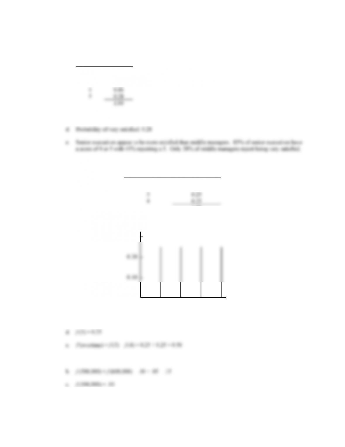
The total number of responses is 1014, so f(0) = 365/1014 = .3600; f(1) = 264/1014 = .2604;
and so on.
x
f (x)
xf (x)
x –
(x –
)2
(x –
)2 f (x)
0
0.3600
0.0000
-1.3087
1.7126
0.6165
1
0.2604
0.2604
-0.3087
0.0953
0.0248
2
0.1903
0.3807
0.6913
0.4779
0.0910
3
0.0897
0.2692
1.6913
2.8606
0.2567
4
0.0996
0.3984
2.6913
7.2432
0.7215
Total
1.0000
1.3087
1.7104
d. The possible values of y are 1, 2, 3, and 4. The total number of responses is 649, so f(1) = 264/649 =
.41; f(2) = 193/649 = .30; and so on.
y
f (y)
yf (y)
1
.4068
.4068
2
.2974
.5948
3
.1402
.4206
4
.1556
.6225
Total
1.0000
2.0447
cup of coffee on an average day is 2.0447 or approximately a mean of 2 cups per day. As expected,
the mean is somewhat higher when we only take into account adults that drink at least one cup of
coffee per day.
= 50 (.20) + 150 (.50) + 200 (.30) = 145
Large: E(x) = x f (x)
b. Medium
x
f (x)
x –
(x –
)2
(x –
)2 f (x)
50
.20
–95
9025
1805.0
150
.50
5
25
12.5
200
.30
55
3025
907.5
2 = 2725.0
y
f (y)
y –
(y –
)2
(y –
)2 f (y)
0
.20
–140
19600
3920
100
.50
–40
1600
800
300
.30
160
25600
7680
2 = 12,400
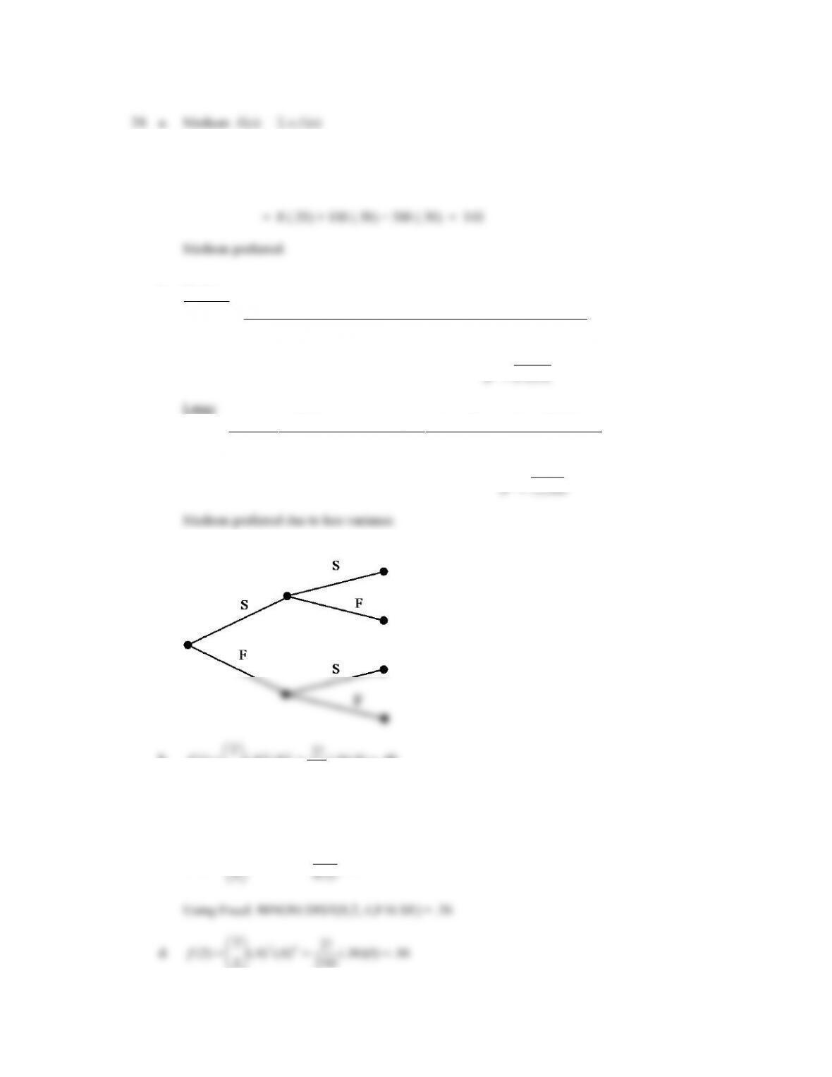
25. a.
b.
11
22!
(1) (.4) (.6) (.4)(.6) .48
11!1!
f
= = =
Using Excel: BINOM.DIST(1,2,.4,FALSE) = .48
c.
02
22!
(0) (.4) (.6) (1)(.36) .36
00!2!
f
= = =
= = =
Using Excel: BINOM.DIST(2,2,.4,FALSE) = .16
e. P(x 1) = f (1) + f (2) = .48 + .16 = .64
b. f (2) = BINOM.DIST(2,10,.1,FALSE) = .1937
c. P(x 2) = f (0) + f (1) + f (2) = .3487 + .3874 + .1937 = BINOM.DIST(2,10,.1,TRUE) = .9298
d. P(x 1) = 1 – f (0) = 1 – .3487 = .6513
b. f (16) = BINOM.DIST(16,20,.7,FALSE) = .1304
c. P(x 16) = 1 – BINOM.DIST(15,20,.7,TRUE) = .2375
d. P(x 15) = 1 – P (x 16) = 1 – .2375 = .7625
=
4.2
= 2.0494