62. The data in ascending order follow.
Position
Value
Position
Value
1
0
11
3
2
0
12
3
3
1
13
3
4
1
14
4
5
1
15
4
6
1
16
5
7
1
17
5
8
2
18
6
9
3
19
6
10
3
20
7
a. The mean is 2.95 and the median is 3.
b.
25
25
( 1) (20 1) 5.25
100 100
p
Ln= + = + =
First quartile or 25th percentile = 1 + . 25(1 1) = 1
75
p
c. The range is 7 and the interquartile range is 4.75 – 1 = 3.75.
63. a.
50
( ) (23) 11.5
100 100
p
in= = =
(12th position)
Previous Coach Median = 850,000
New Coach Median = 1,150,000
b. Range: Previous Coach Base: 3,500,000 – 267,800 = 3,232,200
z−
213
()2.2209 10 1,004,740
i
xx x
−
1 22
−
d. The new coaches have a higher median annual salary, but a smaller range and standard deviation.
64. a. The mean and median patient wait times for offices with a wait tracking system are 17.2 and 13.5,
respectively. The mean and median patient wait times for offices without a wait tracking system are
29.1 and 23.5, respectively.
d.
37 29.1 0.48
16.6
z−
==
37 17.2 2.13
65. a.
148 7.4
20
i
x
xn
= = =
( 1) 19
−
66. a.
20665 413.3
50
i
x
xn
= = =
This is slightly higher than the mean for the study.
b.
2
()69424.5 37.64
( 1) 49
i
xx
sn
−
= = =
−
25
p
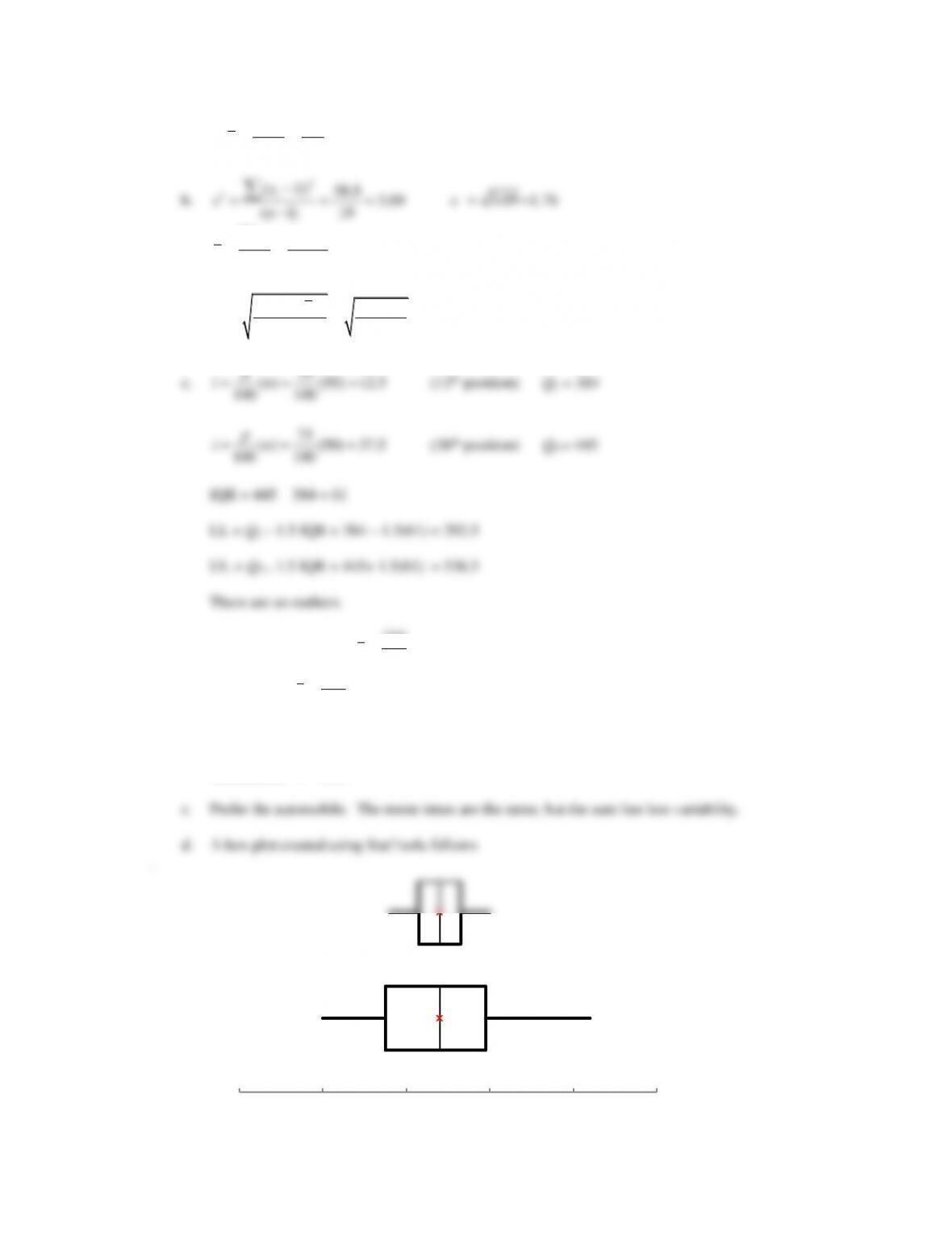
67. a. Public Transportation:
x= =
320
10 32
Automobile:
x= =
320
10 32
b. Public Transportation: s = 4.64
Automobile: s = 1.83

The box plot shows lower variability with automobile transportation and supports the conclusion in
part c.
68. a. The data in ascending order follow:
Median or 50th percentile = 52.1 + . 5(52.1 52.1) = 52.1
b. Percentage change =
52.1 55.5 100 6.1%
55.5
−
=−
c.
25
25
( 1) (14 1) 3.75
100 100
p
Ln= + = + =
25th percentile = 49.4 + .75(51.2 49.4) = 50.75
75
p
Using this approach the first observation (46.5) and the last observation (64.5) would be consider
outliers.
The two approaches will not always provide the same results.
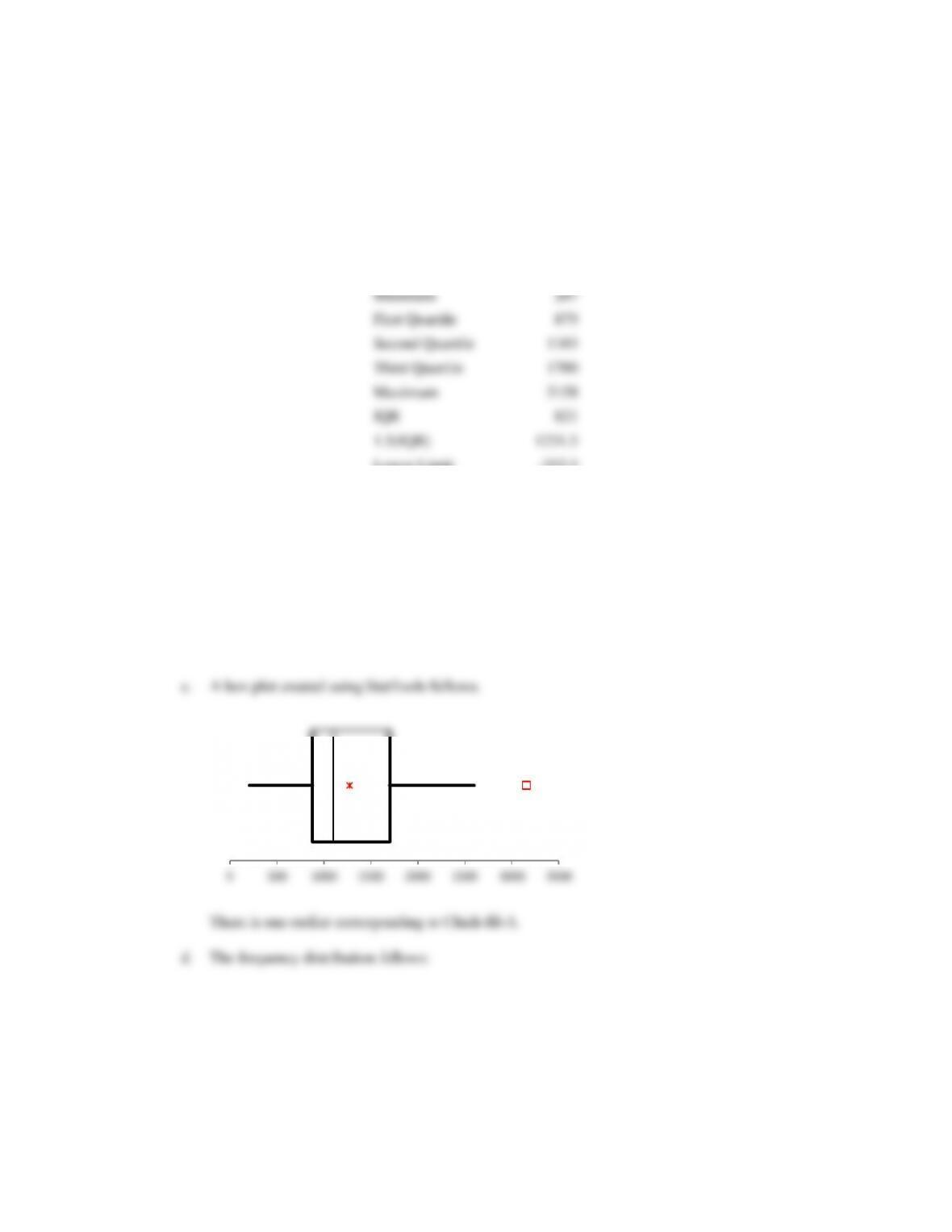
69. Excel’s MIN, QUARTILE.EXC, and MAX functions provided the following results; values for the
IQR and the upper and lower limits are also shown.
Poverty %
Minimum
207
First Quartile
879
Second Quartile
1103
Third Quartile
1700
Maximum
3158
IQR
821
1.5(IQR)
1231.5
Lower Limit
-352.5
Upper Limit
2931.5
a. Mean = 1275.2
b. First quartile = 879 and the third quartile = 1700
25% of the restaurants have an average sales per unit less than or equal to 879 and 25% of the
restaurants have an average sales per unit greater than or equal to 1700.
The frequency distribution shows that the lowest average sales per unit is for the Pizza/Pasta
segment.
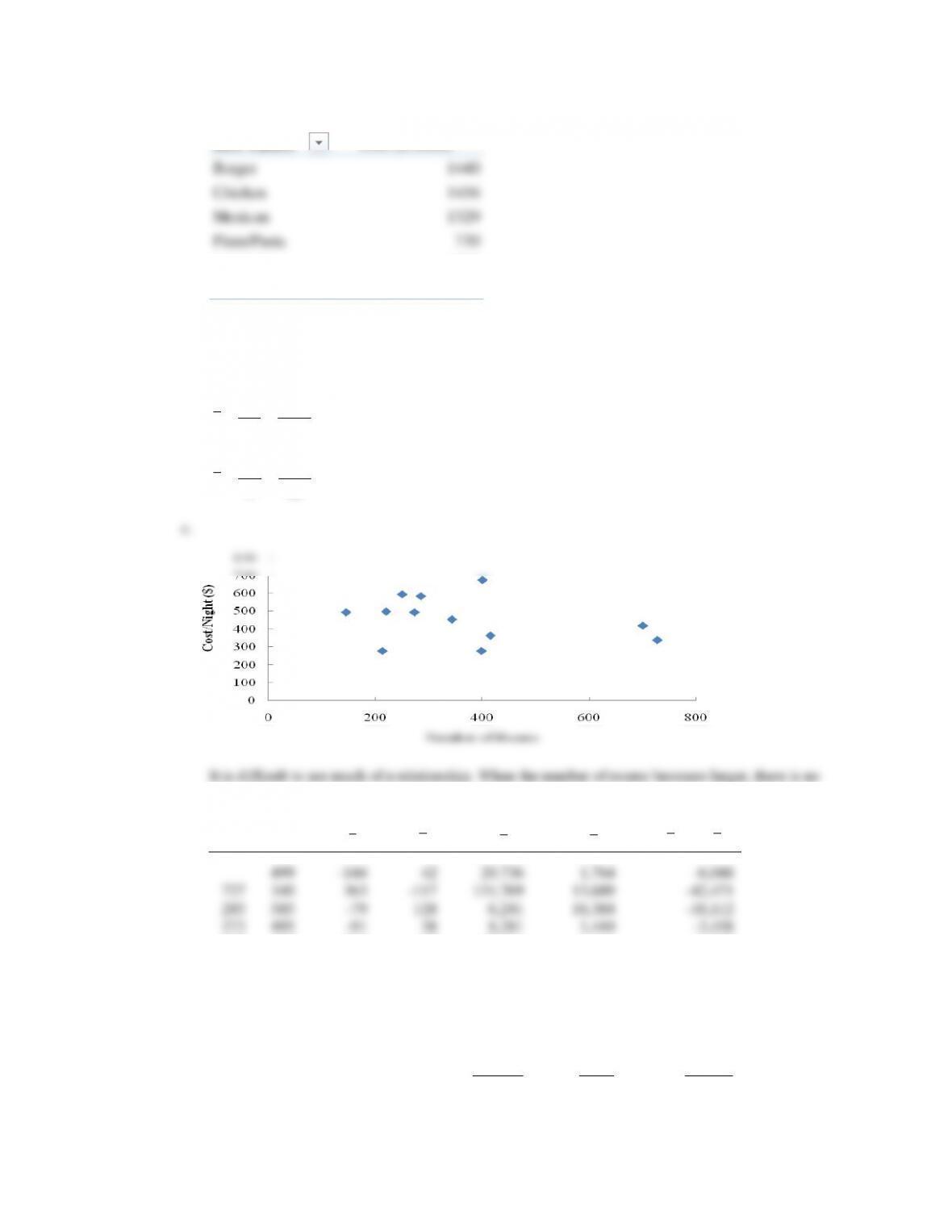
70. a.
4368 364
12
i
x
xn
= = =
rooms
b.
5484 $457
12
i
y
yn
= = =
indication that the cost per night increases. The cost per night may even decrease slightly.
d.
499
–144
42
20.736
1,764
-6,048
727
340
–117
13,689
-42,471
285
585
–79
128
6,241
16,384
-10,112
Row Labels
Average Sales per
Unit ($1000s)
Burger 1440
Chicken 1456
Mexican 1329
Pizza/Pasta 730
Sandwich 1280
Snacks 1088
Grand Total 1275
i
x
i
y
()
i
xx−
()
i
yy−
2
()
i
xx−
2
()
i
yy−
( )( )
ii
x x y y−−
273
495
–91
38
8,281
1,444
-3,458
145
495
–219
38
47,961
1,444
-8,322
213
279
–151
–178
22,801
31,684
26,878
398
279
34
–178
1,156
31,684
-6,052
343
455
–21
-2
441
4
42
250
595
–114
138
12,996
19,044
-15,732
414
367
50
–90
2,500
8,100
-4,500
400
675
36
218
1,296
47,524
7,848
700
420
336
–37
112,896
1,369
-12,432
2
2
( )( ) 74,350 6759.91
1 11
()369,074 183.17
1 11
()174,134 125.82
1 11
6759.91 .293
(183.17)(125.82)
ii
xy
i
x
i
y
xy
xy
xy
x x y y
sn
xx
sn
yy
sn
s
rss
− − −
= = = −
−
−
= = =
−
−
= = =
−
−
= = = −
There is evidence of a slightly negative linear association between the number of rooms and the cost
per night for a double room. Although this is not a strong relationship, it suggests that the higher
room rates tend to be associated with the smaller hotels.
This tends to make sense when you think about the economies of scale for the larger hotels. Many
of the amenities in terms of pools, equipment, spas, restaurants, and so on exist for all hotels in the
Travel + Leisure top 50 hotels in the world. The smaller hotels tend to charge more for the rooms.
The larger hotels can spread their fixed costs over many room and may actually be able to charge
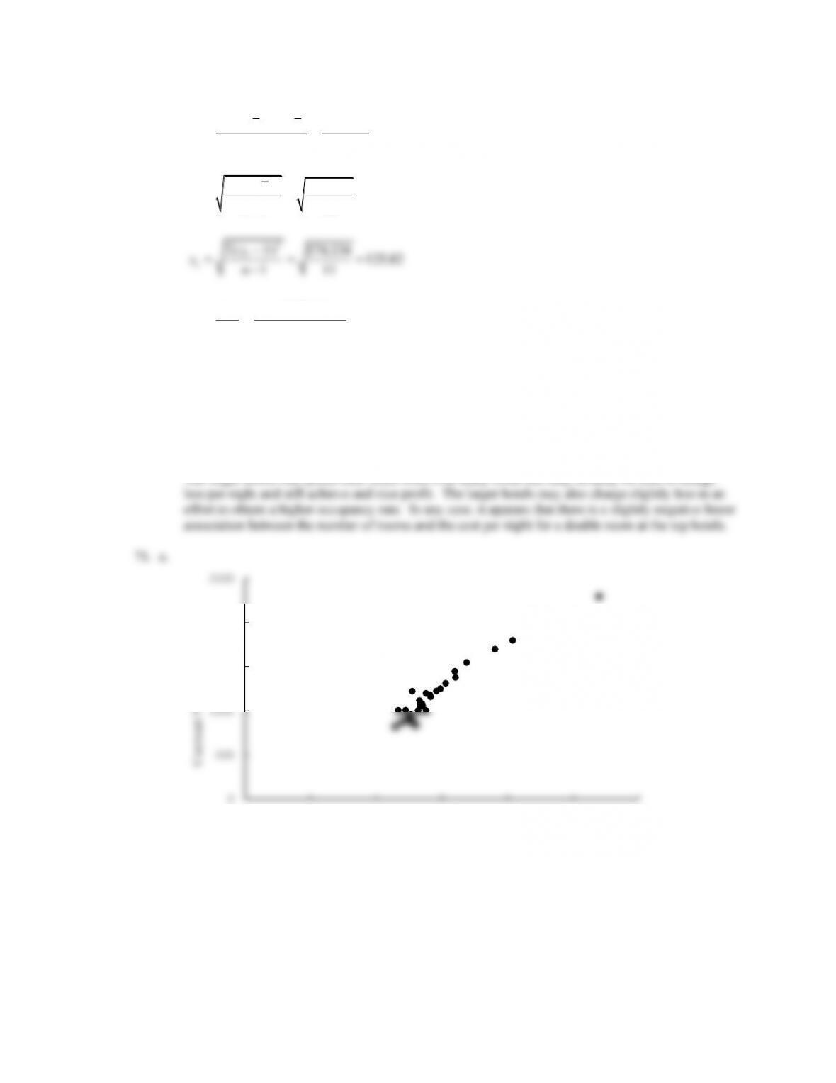
There appears to be a positive linear relationship between two variables.
b. Using Excel’s CORREL function the sample correlation coefficient is .96. This indicates a very
strong linear relationship between the two variables.
72. a.
500
1000
1500
2000
2500
0100 200 300 400 500 600
Current Value ($ millions)
Revenue ($ millions)

i
x
i
y
()
i
xx−
()
i
yy−
2
()
i
xx−
2
()
i
yy−
( )( )
ii
x x y y−−
.407
.422
-.1458
-.0881
.0213
.0078
.0128
.429
.586
-.1238
.0759
.0153
.0058
-.0094
.417
.546
-.1358
.0359
.0184
.0013
-.0049
.569
.500
.0162
-.0101
.0003
.0001
-.0002
.569
.457
.0162
-.0531
.0003
.0028
-.0009
.533
.463
-.0198
-.0471
.0004
.0022
.0009
.724
.617
.1712
.1069
.0293
.0114
.0183
.500
.540
-.0528
.0299
.0028
.0009
-.0016
.577
.549
.0242
.0389
.0006
.0015
.0009
.692
.466
.1392
-.0441
.0194
.0019
-.0061
.500
.377
-.0528
-.1331
.0028
.0177
.0070
.731
.599
.1782
.0889
.0318
.0079
.0158
.643
.488
.0902
-.0221
.0081
.0005
-.0020
.448
.531
-.1048
.0209
.0110
.0004
-.0022
Total
.1617
.0623
.0287
( )( ) .0287 .0022
1 14 1
ii
xy
x x y y
sn
− −
= = =
−−
2
().1617 .1115
1 14 1
i
x
xx
sn
−
= = =
−−
2
().0623 .0692
1 14 1
i
y
yy
sn
−
= = =
−−
.0022 .286
xy
s
during spring training and its winning percentage during the regular season. The spring training
record should not be expected to be a good indicator of how a team will play during the regular
season.
73.
20(20) 30(12) 10(7) 15(5) 10(6) 965 11.4
20 30 10 15 10 85
ii
i
wx
xw
+ + + +
= = = =
+ + + +
days
74.
wi
xi
wi xi
i
xx−
2
()
i
xx−
2
()
ii
w x x−
10
47
470
-13.68
187.1424
1871.42
40
52
2080
-8.68
75.3424
3013.70
150
57
8550
-3.68
13..5424
2031.36
175
62
10850
+1.32
1.7424
304.92
75
67
5025
+6.32
39.9424
2995.68
15
72
1080
+11.32
128.1424
1922.14
10
77
770
+16.32
266.3424
2663.42
475
28,825
14,802.64
a.
28,825 60.68
475
x==
214,802.64 31.23
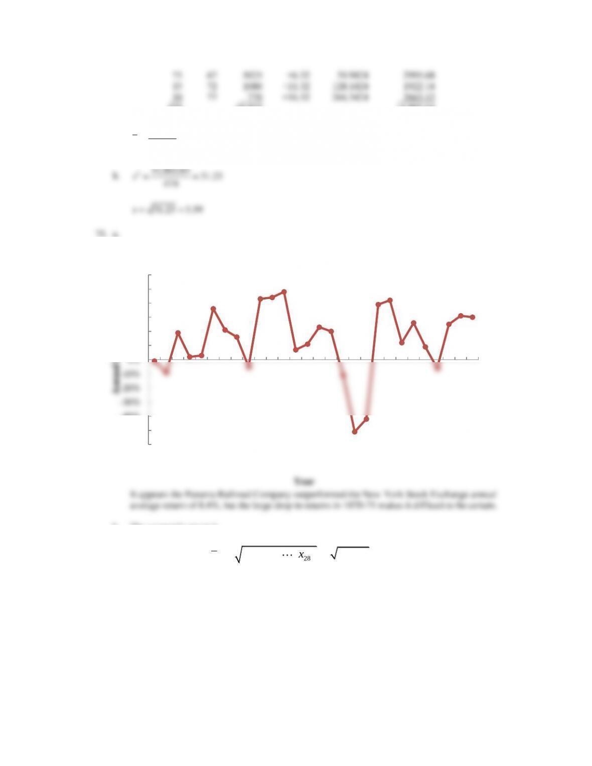
b. The geometric mean is
( )( ) ( )
28
28 1 2 28 16.769 1.106
g
x x x x= = =
So the mean annual return on Panama Railroad Company stock is 10.6%. During the period of
1853–1880, the Panama Railroad Company stock yielded a return superior to the 8.4% earned by the
New York Stock Exchange.
Note that we could also calculate the geometric mean with Excel. If the growth factors for the
individual years are in cells C2:C30, then typing =GEOMEAN(C2:C30) into an empty cell will yield
the geometric mean.