
Chapter 3
Descriptive Statistics: Numerical Measures
Learning Objectives
1. Understand the purpose of measures of location.
2. Be able to compute the mean, weighted mean, geometric mean, median, mode, quartiles, and various
percentiles.
3. Understand the purpose of measures of variability.
4. Be able to compute the range, interquartile range, variance, standard deviation, and coefficient of
variation.
5. Understand skewness as a measure of the shape of a data distribution. Learn how to recognize when a
data distribution is negatively skewed, roughly symmetric, and positively skewed.
6. Understand how z scores are computed and how they are used as a measure of relative location of a
data value.
7. Know how Chebyshev’s theorem and the empirical rule can be used to determine the percentage of
the data within a specified number of standard deviations from the mean.
8. Learn how to construct a 5–number summary and a box plot.
9. Be able to compute and interpret covariance and correlation as measures of association between two
variables.
10. Understand the role of summary measures in data dashboards.
Solutions:
1.
xx
n
i
= = =
75
515
2.
xx
n
i
= = =
96
616
3. a.
xw x
w
i i
i
= = + + +
+ + + = =
6 32 3 2 2 25 8 5
6 3 2 8
702
19 369
( . ) ( ) ( . ) ( ) . .
32 2 25 5
12 7
. . . .
+ + + = =
Period
Rate of Return (%)
1
-6.0
2
-8.0
3
-4.0
4
2.0
5
5.4
The mean growth factor over the five periods is:
( )( ) ( ) ( )( )( )( )( )
5
5
1 2 5 0.940 0.920 0.960 1.020 1.054 0.8925 0.9775
n
g
x x x x= = = =
b. The median commute time is 25.95 minutes.
c. The data are bimodal. The modes are 23.4 and 24.8.
firms in Atlanta is slightly lower than the median salary reported by the Wall Street Journal.
b.
1260 84
15
i
x
xn
= = =
Mean salary is $84,000. The sample mean salary for the sample of 15 middle-level managers is
greater than the median salary. This indicates that the distribution of salaries for middle-level
53
55
63
67
73
75
77
80
83
85
93
106
108
118
124
25
( 1) (16) 4
100 100
p
in= + = =
9. a.
148 14.8
10
i
x
xn
= = =
b. Order the data from low 6.7 to high 36.6
6.7, 7.2, 7.2, 7.6, 10.1, 16.1, 16.4, 17.2, 22.9, 36.6
50
p
75
p
The percentage of total endowments held by these 2.3% of colleges and universities is
(148/413)(100) = 35.8%.
• Hiring freezes for faculty and staff
• Delaying or eliminating construction projects
20
Order the data from the lowest rating (42) to the highest rating (83)
Position
Rating
Position
Rating
1
42
11
67
2
53
12
67
3
54
13
68
4
61
14
69
5
61
15
71
6
61
16
71
7
62
17
76
8
63
18
78
9
64
19
81
10
66
20
83
First quartile or 25th percentile = 61
75
75
( 1) (20 1) 15.75
100 100
p
Ln= + = + =
90th percentile = 78 + .9(81 78) = 80.7
90% of the ratings are 80.7 or less;10% of the ratings are 80.7 or greater.
c. The median number of hours worked per week for high school science teachers is greater than the
median number of hours worked per week for high school English teachers; the difference is 54 – 47
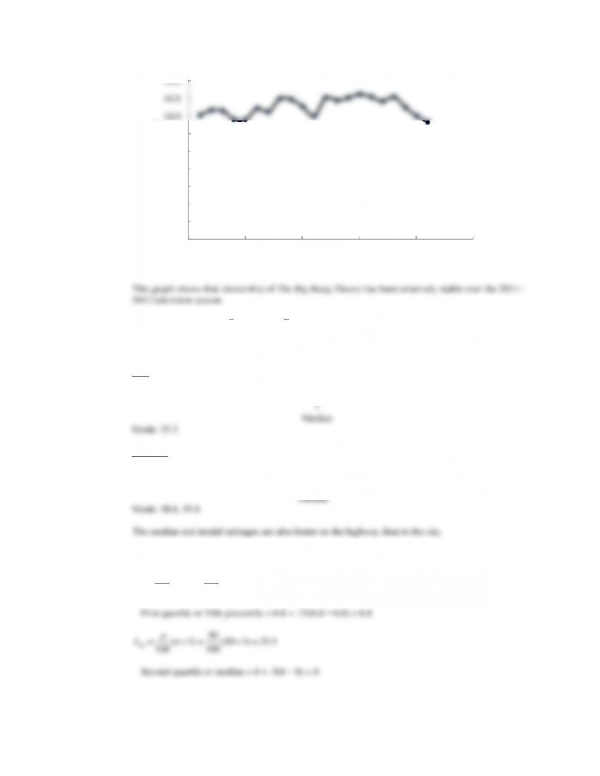
b. The mean number of viewers that watched a new episode is 15.04 million or approximately 15.0
million; the median also 15.0 million. The data is multimodal (13.6, 14.0, 16.1, and 16.2 million); in
such cases the mode is usually not reported.
13. Using the mean we get
xcity
=15.58,
highway
x
= 18.92
For the samples we see that the mean mileage is better on the highway than in the city.
City
13.2 14.4 15.2 15.3 15.3 15.3 15.9 16 16.1 16.2 16.2 16.7 16.8
Highway
17.2 17.4 18.3 18.5 18.6 18.6 18.7 19.0 19.2 19.4 19.4 20.6 21.1
14. For March 2011:
25
25
( 1) (50 1) 12.75
100 100
p
Ln= + = + =
0.0
2.0
4.0
6.0
8.0
10.0
12.0
14.0
16.0
18.0
0 5 10 15 20 25
Viewers (millions)
Period
75
75
( 1) (50 1) 38.25
100 100
p
Ln= + = + =
Third quartile or 75th percentile = 9.4 + . 25(9.6 9.4) = 9.45
For March 2012:
75
p
25
p
It may be easier to compare these results if we place them in a table.
March 2011
March 2012
First Quartile
6.80
6.20
Median
8.00
7.35
Third Quartile
9.45
8.60
The results show that in March 2012 approximately 25% of the states had an unemployment rate of
15. To calculate the average sales price we must compute a weighted mean. The weighted mean is
( ) ( ) ( ) ( ) ( ) ( ) ( ) ( )
501 34.99 1425 38.99 294 36.00 882 33.59 715 40.99 1088 38.59 1644 39.59 819 37.99
501 1425 294 882 715 1088 1644 819
+ + + + + + +
+ + + + + + +
= 38.11
16. a.
Grade xi
Weight wi
4 (A)
9
3 (B)
15
2 (C)
33
1 (D)
3
0 (F)
0
60 Credit Hours
9(4) 15(3) 33(2) 3(1) 150 2.50
9 15 33 3 60
ii
i
wx
xw
+ + +
= = = =
+ + +
b. Yes; satisfies the 2.5 grade point average requirement
17. a.
9191(4.65) 2621(18.15) 1419(11.36) 2900(6.75)
9191 2621 1419 2900
ii
i
wx
xw
+ + +
== + + +
126,004.14 7.81
16,131
==
The weighted average total return for the Morningstar funds is 7.81%.
18.
Assessment
Deans
wixi
Recruiters
wixi
5
44
220
31
155
4
66
264
34
136
3
60
180
43
129
2
10
20
12
24
1
0
0
0
0
Total
180
684
120
444
ii
wx
684 3.8
ii
wx
factors:
Year
% Growth
Growth Factor xi
2010
5.5
1.055
2011
1.1
1.011
2012
-3.5
0.965
2013
-1.1
0.989
2014
1.8
1.018
Stivers
Trippi
Year
End of Year
Value
Growth
Factor
End of Year
Value
Growth
Factor
2004
$11,000
1.100
$5,600
1.120
2005
$12,000
1.091
$6,300
1.125
2006
$13,000
1.083
$6,900
1.095
2007
$14,000
1.077
$7,600
1.101
2008
$15,000
1.071
$8,500
1.118
2009
$16,000
1.067
$9,200
1.082
2010
$17,000
1.063
$9,900
1.076
2011
$18,000
1.059
$10,600
1.071
For the Stivers mutual fund we have:
18000=10000
( )( ) ( )
1 2 8
x x x
, so
( )( ) ( )
1 2 8
x x x
=1.8 and
( )( ) ( )
8
1 2 8 1.80 1.07624
n
g
x x x x= = =
So the mean annual return for the Stivers mutual fund is (1.07624 – 1)100 = 7.624%
For the Trippi mutual fund we have:
( )( ) ( )
1 2 8
x x x
( )( ) ( )
1 2 8
x x x
( )( ) ( )
9
1 2 9 1.428571 1.040426
n
g
x x x x= = =
( )( ) ( )
6
1 2 6 2.50 1.165
n
g
x x x x= = =
10, 12, 16, 17, 20
25
25
( 1) (5 1) 1.5
100 100
p
Ln= + = + =
First quartile or 25th percentile = 10 + . 5(12 10) = 11
75
p
n
515
sx x
n
i
22
1
64
416=−
−= =
( )
25. 15, 20, 25, 25, 27, 28, 30, 34 Range = 34 – 15 = 19
25
25
( 1) (8 1) 2.25
100 100
p
Ln= + = + =
First quartile or 25th percentile = 20 + . 25(20 15) = 21.25
75
75
( 1) (8 1) 6.75
100 100
p
Ln= + = + =
Mean
3.72
Standard Error
0.0659
Median
3.605
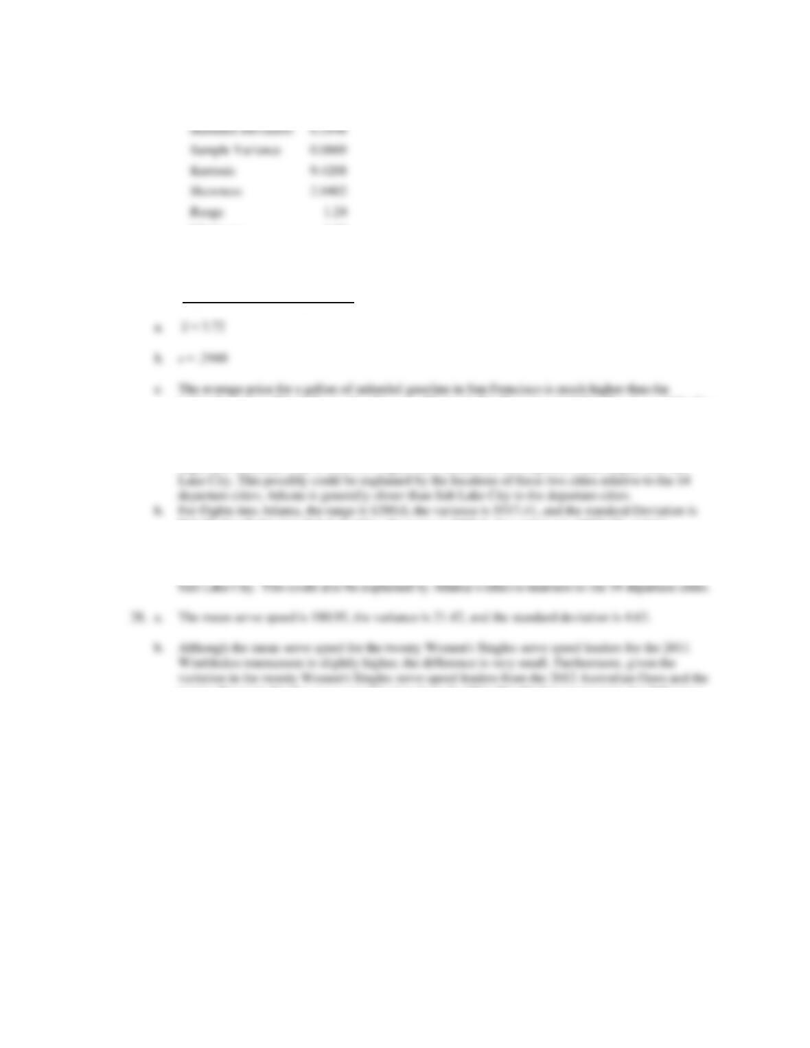
Mode
3.59
Standard Deviation
0.2948
Sample Variance
0.0869
Kurtosis
9.4208
Skewness
2.9402
Range
1.24
Minimum
3.55
Maximum
4.79
Sum
74.4
Count
20
national average. This indicates that the cost of living in San Francisco is higher than it would be for
cities that have an average price close to the national average.
27. a. The mean price for a round–trip flight into Atlanta is $356.73, and the mean price for a round–trip
flight into Salt Lake City is $400.95. Flights into Atlanta are less expensive than flights into Salt
$74.28. For flights into Salt Lake City, the range is $458.8, the variance is 18933.32, and the
standard deviation is $137.60.
The prices for round–trip flights into Atlanta are less variable than prices for round–trip flights into
twenty Women’s Singles serve speed leaders from the 2011 Wimbledon tournament, the difference
in the mean serve speeds is most likely due to random variation in the players’ performances.